Chapter 12 A Brief introduction to MCMC sampling and JAGS
Learning objectives:
- Gain insights into how MCMC sampling works
- Be able to implement your first Bayesian model in JAGS
12.1 Introduction to MCMC sampling
In our moose detection example from Section 11, we could determine the posterior distribution analytically. Usually, we will not be so lucky. In particular, in most cases, there will be no closed form solution to:
\[\begin{equation} p(\theta | y) = \frac{L(y | \theta)\pi(\theta)}{\int_{-\infty}^{\infty}L(y | \theta)\pi(\theta)} \end{equation}\]
Instead, we will generate samples that we can use to summarize the posterior distribution, \(p(\theta | y)\). There are many ways to generate a sample from the posterior distribution. In this section, we will briefly consider one possible way to generate a Markov chain (an autocorelated sequence of parameter values) that converges in distribution to \(p(\theta|y)\). This approach, called Metropolis, is one of many possible Markov Chain Monte Carlo (MCMC) approaches used to generate samples from a posterior distribution.
12.2 Metropolis algorithm
MCMC approaches generate a sequence of parameter values using a set of rules that allow the sampler to explore the full range of support of the posterior distribution, while spending most of the time in areas where the posterior distribution is at its highest point (Fig. 12.1).
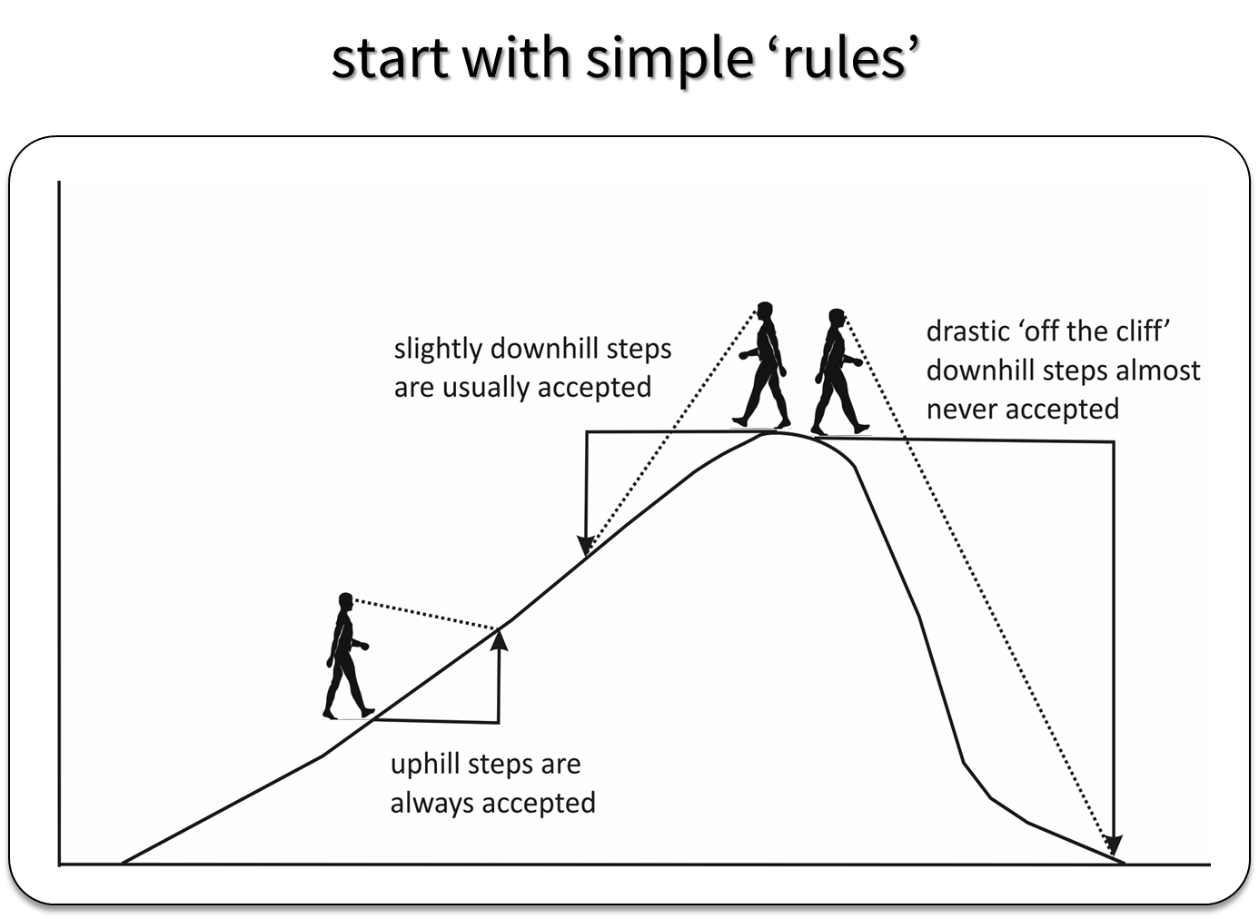
FIGURE 12.1: Depiction of how the Metropolis Algorithm works. Figure created by Evan Cooch, Cornell University.
Remember, the posterior distribution is given by:
\[\begin{equation} p(\theta | y) = \frac{L(y | \theta)\pi(\theta)}{\int_{-\infty}^{\infty}L(y | \theta)\pi(\theta)} \end{equation}\]
Consider two possible values of \(\theta\) = {\(\theta_1\) and \(\theta_2\)}. Without the denominator, we cannot evaluate \(p(\theta_1 | y)\) or \(p(\theta_2 | y)\). We can, however, evaluate the relative likelihood, \(R\) of \(\theta_1\) and \(\theta_2\) since the denominator will cancel out:
\[\begin{equation} R = \frac{p(\theta_2 | y)}{p(\theta_1 | y)} = \frac{L(y | \theta_2)\pi(\theta_2)}{L(y | \theta_1)\pi(\theta_1)} \end{equation}\]
The Metropolis algorithm uses this relative likelihood to determine a sequence of parameter values using the following algorithm:
Initiate the Markov chain with an initial starting value, \(\theta_0\)
Generate a new, proposed value of \(\theta\) from a symmetric distribution centered on \(\theta_0\) (e.g., \(\theta^{\prime}\) = rnorm(\(\theta_0, \sigma\))).
Decide whether to accept or reject \(\theta^{\prime}\):
If R = \(\frac{p(\theta^{\prime} | y)}{p(\theta_0 | y)} > 1\), we move up the probability hill in Figure 12.1 and accept the proposed value, setting \(\theta_1 = \theta^{\prime}\).
If R \(<1\), the proposal moves us down the probability hill. In this case, we accept \(\theta^{\prime}\) with probability = R. To do so, we generate a uniform random number, \(u\), between 0 and 1. If \(u \le R\), then we accept the new value, setting \(\theta_1=\theta^{\prime}\). Otherwise, we reject the new value and keep \(\theta_1\) at \(\theta_0\).
Return to step 2, replacing \(\theta_0\) with \(\theta_1\).
Note that step 3 ensures that the proposed parameter values that move us up the probability hill (towards higher values of the posterior distribution) are always accepted, but also that we do not get stuck at the top of the hill (i.e., we continue to sample from the full range of parameters supported by the posterior distribution). This strategy is not too difficult to program - if you want to see what R code would look like for a Metropolis sampler, see: https://theoreticalecology.wordpress.com/2010/09/17/metropolis-hastings-mcmc-in-r/.
We will continue to sample until:
The distribution of \(\theta_1, \theta_2, \ldots, \theta_M\) appears to have reached a steady state (i.e., the chain has converged to an equilibrium distribution).
The MCMC sample, \(\theta_1, \theta_2, \ldots, \theta_M\), is large enough that we can summarize characteristics of \(p(\theta | data)\) (e.g., its mean, median, 2.5th and 97.5th quantiles) to our desired level of precision.
An example Markov Chain may look something like Figure 12.2. This plot is called a traceplot, and it depicts the series of parameter values generated using MCMC sampling for 4 different parameters (represented in the different panels of the plot). In this case, two different Markov chains (shown in red and blue) were initiated at different starting values. Eventually, the two chains converge in distribution as evidenced by the red and blue plots largely overlapping after the first set of 500-1000 samples. Usually, we will discard the initial parameter values where the chains are clearly sampling different regions of the parameter space, which we label as a “burn-in” period.
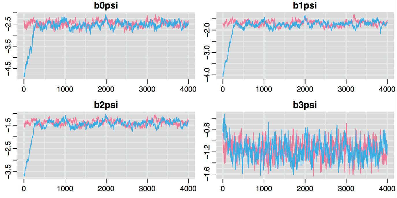
FIGURE 12.2: Traceplot depicting the series of parameter values generated using MCMC sampling. Two different Markov chains are shown in red and blue. These chains were initiated at different starting values, but converge in distribution after an initial burn in period.
Once we have these samples, we can estimate \(\theta\) by the mean (or median) of the samples, and we can compute credible intervals using quantiles of the sampled values.
How do we know if we have sampled long enough - i.e., that our sample has converged in distribution to \(p(\theta|y)\)? The short answer is that there is no foolproof method for detecting convergence. Some things that we can and will do, however, include:
- Run multiple chains (starting in different places) and see if they converge on similar distributions
- Discard the first \(n_{burnin}\) iterations (where the sampler has not yet converged)
- Consider the Gelman-Rubin Statistic (Gelman, Rubin, & others, 1992), Rhat, which is output by JAGS. Rhat compares the variance of parameter values between chains to the variance of parameter values within chains. Values near 1 suggest likely convergence. As a general rule, Rhat should be less than 1.1.
12.3 Aside: Sampler performance
With Metropolis or Metropolis-Hastings (the latter allows for non-symmetric proposal distributions), we need to consider how to generate good proposals for our parameters (i.e., “candidate” parameter values during step 2 of the process). This may require setting one or more “tuning” parameters to ensure the sampler does not get stuck at the top of the hill or jump too far away from the current value that we miss the hill altogether. For example, when using the normal distribution, we can try different values of \(\sigma\) and pick a value that ensures steps are big enough that we efficiently sample all areas of the posterior distribution without being so big that we completely “fall off the cliff” when we are at the top of the hill (Fig. 12.1).
In this book, we will be using JAGS (Plummer & others, 2003) to implement Bayesian models. There are a number of packages available to run JAGS from within R (e.g., rjags , runjags, R2jags, rube, etc); we will generally use R2Jags (Su & Masanao Yajima, 2021). JAGS has a variety of different MCMC algorithms at its disposal, and it will attempt to determine the best algorithm depending on the likelihood and set of prior distributions (one for each parameter) we supply it. Although JAGS is quite powerful, there are other approaches developed in recent years, not available in JAGS, that are more efficient (i.e., reach steady state quicker and better explore the distribution of \(p(\theta | data)\)). For example, STAN (Carpenter et al., 2017), a popular alternative to JAGS, employs a “No-U-Turn” (NUTS) sampler that is typically more efficient at sampling the posterior distribution (Hoffman & Gelman, 2014); for a visual demonstration of different samplers, see http://elevanth.org/blog/2017/11/28/build-a-better-markov-chain/. STAN can also be run from R (Stan Development Team, 2019), but the syntax is a little more challenging to learn.
12.4 Specifying a model in JAGS
To run a model using JAGS, we will need to:
- Specify prior distributions for all model parameters.
- Specify the likelihood of the data.
- Fit the model by calling JAGS from R to generate samples using its built in MCMC routines.
- Evaluate whether or not we think the samples have converged in distribution to \(p(\theta | y)\).
- Use our samples to characterize the posterior distribution, \(p(\theta | data)\).
Let’s revisit our linear model for comparing the mean jaw lengths of male and female golden jackals from Section 3.5.1. The data are again provided, below:
males<-c(120, 107, 110, 116, 114, 111, 113, 117, 114, 112)
females<-c(110, 111, 107, 108, 110, 105, 107, 106, 111, 111)
As before, we will assume the mean jaw lengths for males and females are normally distributed, with sex-specific means, \(\mu_m\) and \(\mu_f\). We will also, for now, assume that the jaw lengths are equally variable for males and females (Exercise 11.1 will have you will relax this assumption). This leads to the following Likelihood:
- \(y_{males} \sim N(\mu_m, \sigma^2)\)
- \(y_{females} \sim N(\mu_f, \sigma^2)\)
This model has 3 parameters: \(\mu_m, \mu_f,\) and \(\sigma\). We will need to specify prior distributions for each of these parameters. Before doing so, it is important to note that:
- JAGS and WinBugs represent a normal distribution as \(N(\mu, \tau = 1/\sigma^2)\), \(\tau\) is called the precision parameter of the Normal distribution.
- Rather than specify a prior for the precision, it will be easier to specify a prior for \(\sigma\) (this will require thinking about the standard deviation rather than 1/variance). We will then use the prior for the \(\sigma\) to “induce” (i.e., determine) the prior for \(\tau\).
We want to choose priors that are “dispersed” (meaning they allow for a wide range of possible values). One way to do this is to use Normal distributions with large variance parameters (small precision parameters). Alternatively, we can use uniform distributions that allow for a wide range of values. We will use a mix of these strategies, below:
Priors:
- \(\mu_m \sim N(100, 0.001)\)
- \(\mu_f \sim N(100, 0.001)\)
- \(\sigma \sim\) Uniform(0, 30)
JAGS code looks just like R code, but with some differences:
- JAGS code is not executed (it just defines the model)
- It does not matter how we order our code (we can define the prior before likelihood or the likelihood after prior - it will not make a difference).
There are 6 types of objects in JAGS:
Modeled data specified using a \(\sim\) (which can be read as “distributed as”). For example, we will use y \(\sim\) followed by a probability distribution to specify the distribution of our response variable, y, in our regression model.
Unmodeled data: these are objects that are not assigned probability distributions. Examples of unmodeled data include predictors, constants, and index variables used in loops.
Modeled parameters: these are parameters which are given informative priors. These informative priors may also include additional parameters called hyperparameters. Modeled parameters will be used to model what frequentists refer to as random effects. We will not see these until later in the course (Section 18).
Unmodeled parameters: these are parameters that are assigned uninformative priors.
Derived quantities: these are objects determined using the assignment arrow,
<-. For example, we might be interested in obtaining samples for a function of parameters (e.g., \(L_i=L_{\infty}(1-e^{-k(Age_i-t_0)})\) in our bear growth example from Section 10.6). We can accomplish this goal by defining \(L_i\) as a derived quantity, depending on unmodeled data (Age) and modeled parameters (\(L_{\infty}, k, t_0\)).Looping indexes: i, j, used in loops (e.g., over our observations in a data set).
Below, we define our model for the jaw data using a function (by contrast, Kéry (2010) and others often write the model out to a file).
jaw.mod<-function(){

  # Priors
    mu.male ~ dnorm(100, 0.001) # mean of male jaw lengths
    mu.female ~ dnorm(100, 0.001) # mean of female jaw lengths
    sigma ~ dunif(0, 30) # common sigma
    tau <- 1/(sigma*sigma) #precision

  # Likelihood (Y | mu) = normal(mu[gender], sigma^2)
    for(i in 1:nmales){
      males[i] ~ dnorm(mu.male, tau)
    }
    for(i in 1:nfemales){
      females[i] ~ dnorm(mu.female, tau)
    }

  # Derived quantities:  difference in means
    mu.diff <- mu.male - mu.female
}
Here, we can identify the following types of objects in our model:
Modeled data =
males, femalesUnmodeled data =
nmales, nfemalesModeled parameters (none in this example)
Unmodeled parameters =
mu.male, mu.female, sigmaDerived quantities =
tau, mu.diffLooping indexes:
i(used twice)
12.5 Fitting a model using JAGS
We begin by loading the R2jags package as well as the mcmcplots (Curtis, 2018), MCMCvis (Youngflesh, 2018), and ggplot2 (Wickham, 2016) packages to help with visualizing the results.
To begin sampling, JAGS will need a set of initial values (our \(\theta_0\)’s, for example, in step 1 of the Metropolis algorithm). Usually, JAGS can use the prior distributions to generate initial values. This will happen by default unless you supply a set of initial values. Alternatively, you can supply a function to generate initial values (this is the approach Kéry (2010) takes in his book). I tend to be lazy and allow JAGS to generate its own initial values, but this can sometimes get you in trouble (we will see this in a later section).
The function, init.vals, below can be used to generate initial values:
# Function to generate initial values
init.vals<-function(){
    mu.male <- rnorm(1, 100, 100)
    mu.female <- rnorm(1, 100, 100)
    sigma <- runif(1, 0, 10)
    out <- list(mu.male = mu.male, mu.female = mu.female, sigma = sigma)
}
We will also create objects to hold some of the unmodeled data that we will pass to JAGS, namely the number of males and females in the data set.
We then use the jags function to call JAGS and generate our MCMC sample:
t.test.jags <- jags(data=c("males", "females", "nmales",  "nfemales"),
                      inits = init.vals,
                      parameters.to.save = c("mu.male", "mu.female", "sigma", "mu.diff"),
                      progress.bar = "none",
                      n.iter = 10000,
                      n.burnin = 5000,
                      model.file = jaw.mod,
                      n.thin = 1,
                      n.chains = 3)
Note the following arguments:
datawill contain all modeled and unmodeled data (here,malesandfemalescontaining the jaw lengths andnmalesandnfemalescontaining the number of males and females,).parameters.to.saveis a list of parameters for which we want to save the MCMC samples. Here, we specify that we want to keep track of \(\mu_m, \mu_f, \sigma\), and \(\mu_m -\mu_f\). By contrast, we do not save \(\tau\) since we do not intend to examine the posterior distribution of the precision parameter.progress.bar = "none"(for Windows users, you can also try =gui). If we don’t supply this argument, you will get a lot of output in your html file when using Rmarkdown.n.iter = 10000specifies the total number of samples we want to generaten.burnin = 5000specifies that we want to throw away the first 5000 samplesmodel.file = jaw.modspecifies the function containing the model specificationn.thin = 1specifies that we want to keep all of the samples. We can save memory by saving say every other sample if we change this ton.thin = 2. If the chains are highly autocorrelated, we won’t loose much information by keeping every other sample.
n.chains = 3specifies that we want to generate 3 Markov chains, each generated with a different set of starting values.
Alternatively, we could use jags.parallel to take advantage of parallel processing using:
t.test.jags <- jags.parallel(data = c("males", "females", "nmales",  "nfemales"),
                             inits = init.vals,
                             parameters.to.save = c("mu.male", "mu.female", "sigma", "mu.diff"),
                             n.iter = 10000,
                             n.burnin = 5000,
                             model.file = jaw.mod,
                             n.thin = 1,
                             n.chains = 3)
Let’s inspect the output from jags by typing t.test.jags (the name of the object we created).
## Inference for Bugs model at "jaw.mod", fit using jags,
##  3 chains, each with 10000 iterations (first 5000 discarded)
##  n.sims = 15000 iterations saved
##           mu.vect sd.vect    2.5%     25%     50%     75%   97.5%  Rhat n.eff
## mu.diff     4.791   1.497   1.862   3.809   4.795   5.769   7.735 1.001 15000
## mu.female 108.586   1.068 106.492 107.887 108.579 109.272 110.699 1.001 15000
## mu.male   113.376   1.056 111.303 112.680 113.380 114.064 115.503 1.001  9900
## sigma       3.314   0.593   2.389   2.897   3.240   3.648   4.683 1.001 15000
## deviance  103.054   2.733  99.903 101.055 102.374 104.344 110.165 1.001 15000
##
## For each parameter, n.eff is a crude measure of effective sample size,
## and Rhat is the potential scale reduction factor (at convergence, Rhat=1).
##
## DIC info (using the rule, pD = var(deviance)/2)
## pD = 3.7 and DIC = 106.8
## DIC is an estimate of expected predictive error (lower deviance is better).
We see that we get a summary of the posterior distribution for each saved parameter:
mu.vect= the mean of the posterior distributionsd.vect= the standard deviation of the posterior distribution2.5%to97.5%= quantiles of posterior distributionRhatis the Gelman-Rubin statistic for evaluating convergence of the MCMC samples.n.eff= an estimate of the effective sample size. As we will see in a bit, our samples are autocorrelated. This gives us an idea of the equivalent number of samples if we were able to generate parameter values that were independent (i.e., not autocorrelated).
JAGS also returns an estimate of DIC (an information theoretic quantity like AIC that we will briefly discuss in Section 15.7.4).
If we only wanted to view the output for a few select parameters, we can use the MCMCsummary function in the MCMCvis package (Youngflesh, 2018):
##               mean       sd     2.5%      50%    97.5% Rhat n.eff
## mu.male   113.3763 1.056445 111.3029 113.3805 115.5031    1 15206
## mu.female 108.5855 1.068213 106.4917 108.5786 110.6986    1 15237
Before interpreting the output, we should verify that we have sampled long enough that our samples have converged in distribution. Inspecting the values of Rhat, we see that they are all close to 1. It is also a good idea to inspect posterior density plots and trace plots to provide further reassurance that the different chains have ended up in the same spot (see Section 12.6).
We can use the MCMCpstr function in the MCMCvis package to pull off the posterior means to serve as our point estimates and to pull off quantiles of the posterior distribution to form 95% credible intervals.
# Use MCMCsummary to pull off posterior means
bayesests <- MCMCpstr(t.test.jags, params = c("mu.male", "mu.female"), func = mean)
bayesests
## $mu.male
## [1] 113.3763
##
## $mu.female
## [1] 108.5855# Use MCMCsummary to pull of upper and lower 95% credible interval limits
bayesci <- MCMCpstr(t.test.jags, params = c("mu.male", "mu.female"),
func = function(x) quantile(x, probs = c(0.025, 0.975)))
bayesci## $mu.male
## 2.5% 97.5%
## mu.male 111.3029 115.5031
##
## $mu.female
## 2.5% 97.5%
## mu.female 106.4917 110.6986We then fit the same model in a frequentist framework using lm and create a data set with our estimates and credible/confidence intervals.
# Fit linear model in frequentist framework
jawdat<-data.frame(jaws=c(males, females),
                    sex=c(rep("Male", length(males)),
                          rep("Female", length(females))))
lm.jaw<-lm(jaws~sex-1, data=jawdat)
# Store results
betaf <- coef(lm.jaw)
CIf <-confint(lm.jaw)
ests<-data.frame(estimate = c(bayesests$mu.female, bayesests$mu.male, betaf),
                 LCL = c(bayesci$mu.female[1],   bayesci$mu.male[1], CIf[,1]),
                 UCL = c(bayesci$mu.female[2],   bayesci$mu.male[2], CIf[,2]),
                 param = c("Mean females", "Mean males"),
                 Method = rep(c("Bayesian", "Frequentist"), each = 2))
Lastly, we plot the results, showing that they are nearly identical!
ggplot(ests, aes(param,estimate, col = Method)) +
  geom_point(position = position_dodge(width = 0.2))+
  geom_pointrange(aes(ymin = LCL, ymax= UCL), position = position_dodge(width = 0.2))+
  ylab("Estimate") + xlab("") +
  scale_x_discrete(labels = c('Mean females' = expression(mu[f]),
                              'Mean males'   = expression(mu[m]))) +
  scale_colour_colorblind()+
  theme(text = element_text(size = 20))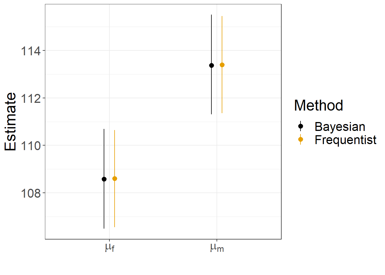
FIGURE 12.3: Comparison of frequentist and Bayesian estimates and confidence/credible intervals for the mean jaw length of male and female jackals.
12.6 Density and traceplots for assessing convergence
When running code in Rstudio, I often like to use the mcmcplot function to visualize output. This function will create a separate html file that you can use to visualize posterior distributions, autocorrelation functions, and traceplots for the different parameters. This function does not work well with bookdown, however, so we will explore these different plots separately.
We can visualize posterior densities using denplot:
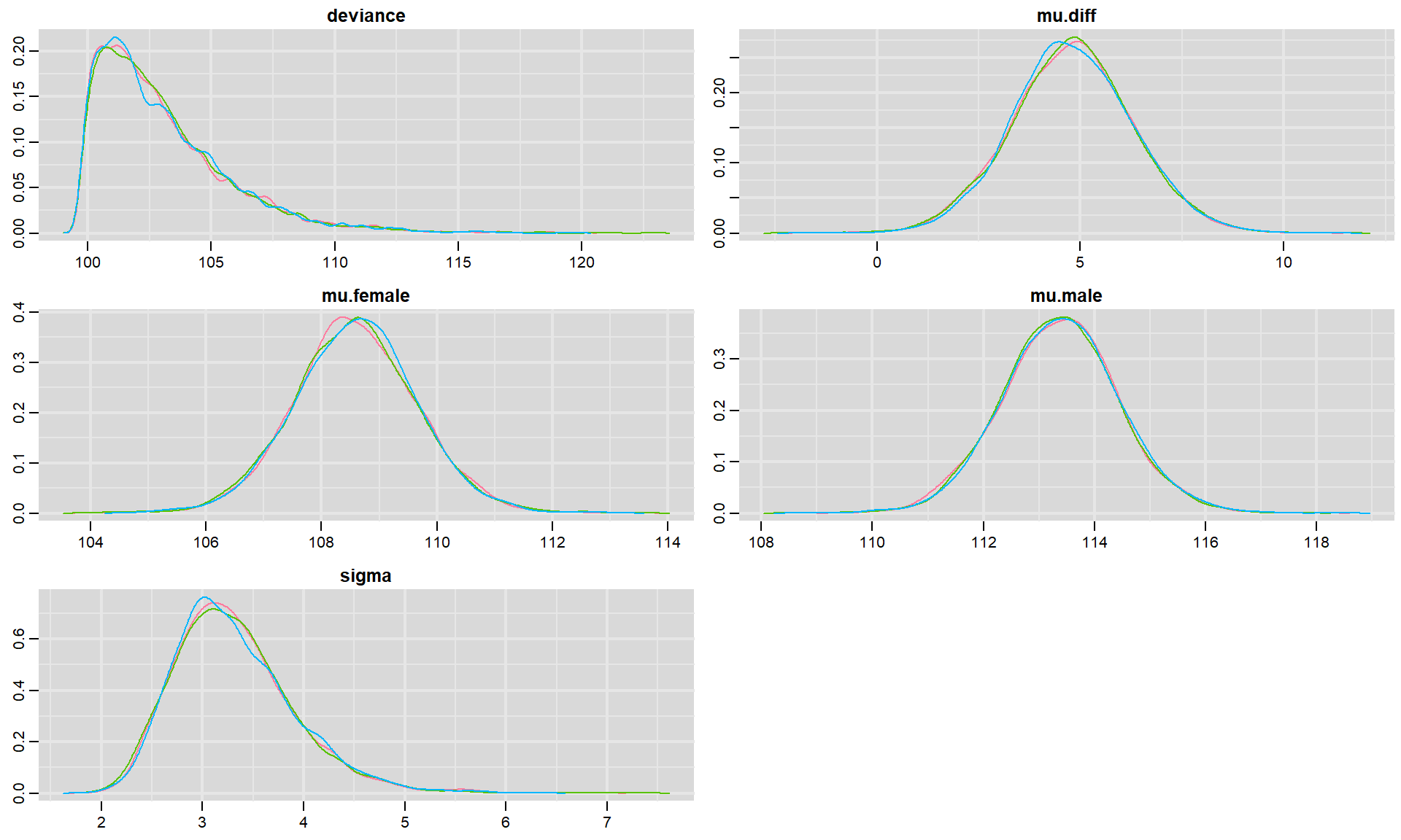
FIGURE 12.4: Posterior density plots for each parameter in our model fit to the jackal jaw lenght data set. Colors in the different panels correspond to different chains.
In each panel, we see density plots for each chain associated with a particular parameter as well as density plots for the deviance (we can also pool results across the different chains if we add collapse = TRUE). For this simple model, it is clear that all three chains ended up in the same place, providing further evidence that we have reached convergence. If we had a large number of parameters, then we could have added the parms argument to provide a list containing a subset of parameters to visualize. For example, we could visualize the posteriors for \(\mu_m\) and \(\mu_f\) usingdenplot(t.test.jags, parms = c("mu.male", "mu.female"))47.
We can also look at traceplots showing the sequence of posterior samples using:
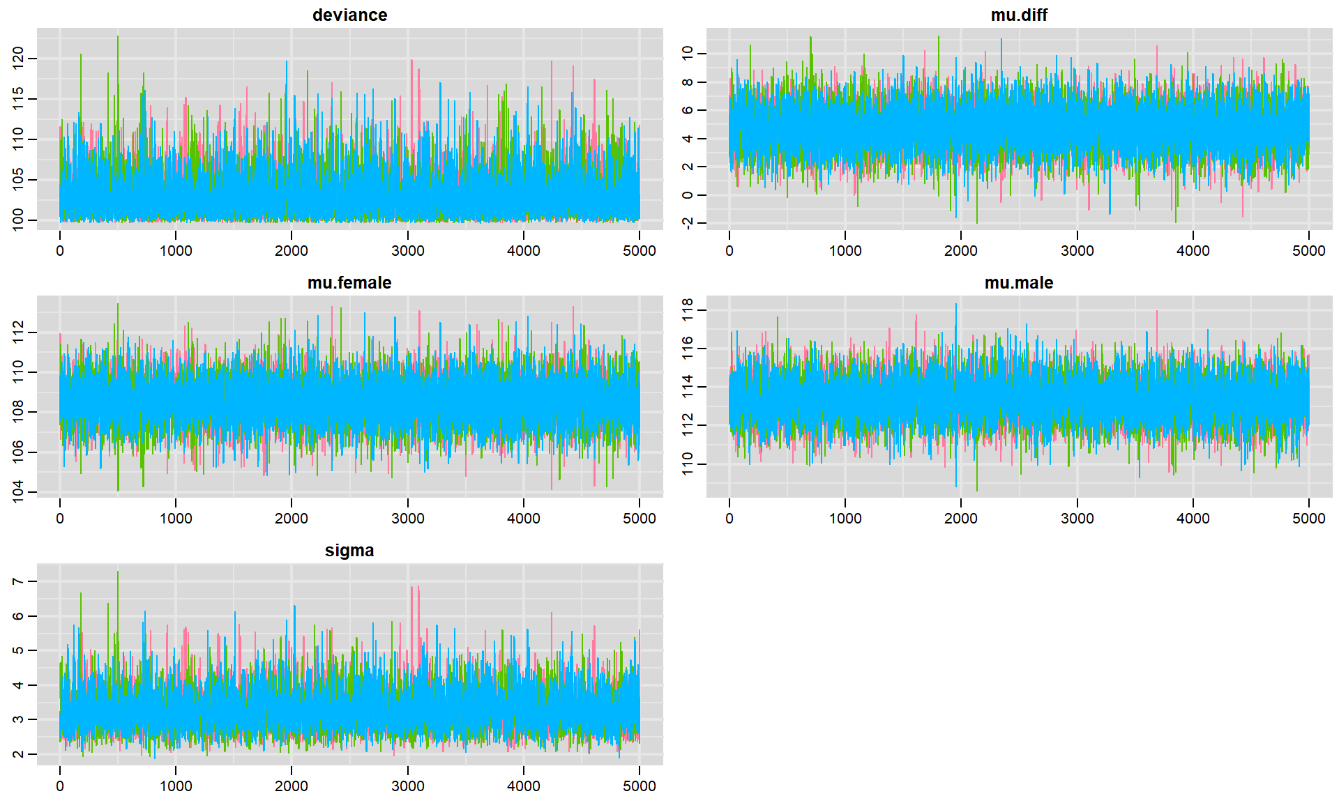
FIGURE 8.2: Trace plots for each parameter in our model fit to the jackal jaw lenght data set. Colors in the different panels correspond to different chains.
Again, the fact that the different chains largely overlap is reassuring. Sometimes, traceplots will not look so noisy - but, rather you will see a slow moving trend over time. The top panels of Fig. 12.2, relative to the bottom right panel give some indication of what I am referring to but the trend may be much more pronounced. When this happens, the samples are highly autocorrelated, and we will have to sample for a long time in order to explore the full range of the posterior distribution. By contrast, these traceplots suggest that the sample is doing a great job quickly exploring the full range of the posterior distribution, and we say the chains are “well mixed”.
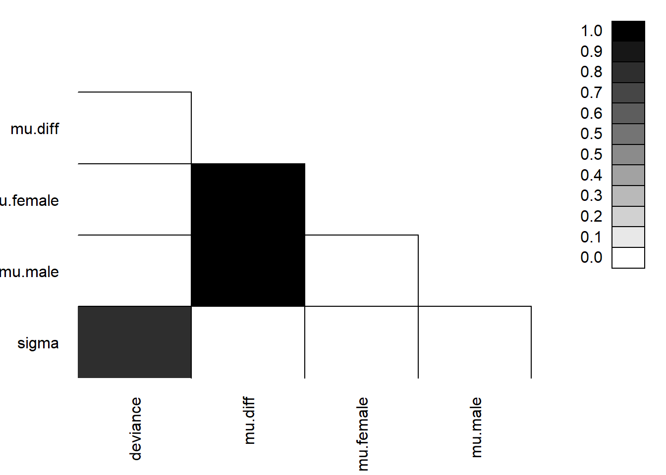
We can look to see if our parameters are correlated with each other using parcorplot.
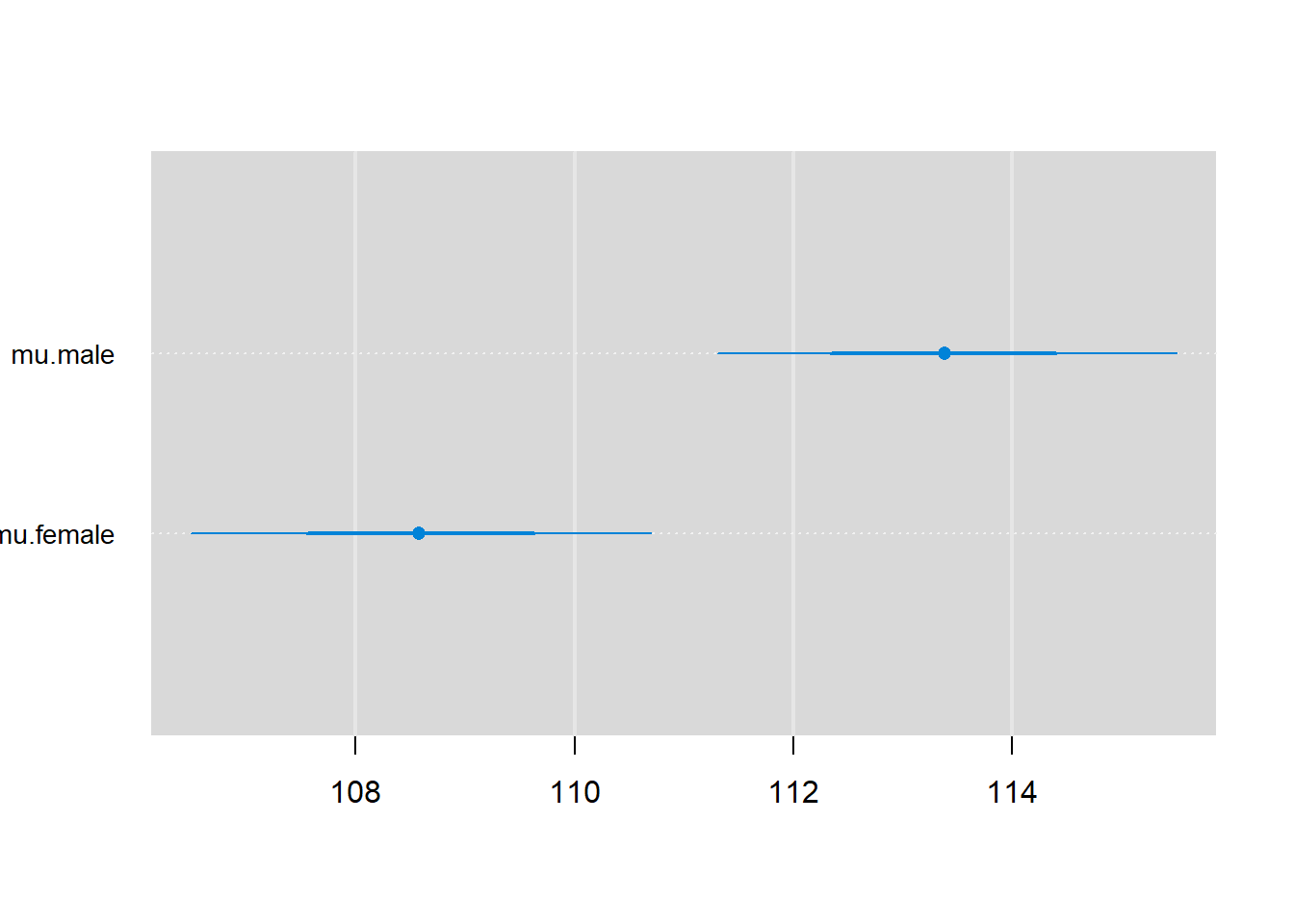
Lastly, we can plot estimates with 68% and 95% credible intervals using caterplot:
Congrats - you have just fit your first JAGS model and learned how to work with and summarize samples from the posterior distribution!
12.7 Tips on running models in JAGS
Kéry (2010) offers lots of good tricks and tips in the Appendix of his book. First and foremost: start simple, then build up towards more complex models! If you have his book, I encourage you to look at his tips numbered: 2, 3, 4, 9, 11, 12 (use %T% in JAGS), 14, 16, 17, 20, 23,24, 25, 26, 27.
Also, as always, googling error messages can be useful for diagnosing problems, and it can help to work together with your peers when learning.
Note, the functions in the
mcmcplotspackage include the argumentparms, whereas the functions in theMCMCvispackage include the argumentparams. It is easy to get these confused. If you use the tab key in Rstudio after typing “par”, you can have the function self-populate with the correct argument.↩