Chapter 14 Introduction to generalized linear models (GLMs)
Learning objectives:
Understand the role of random variables and common statistical distributions in formulating modern statistical regression models
Be able to describe a variety of statistical models and their assumptions using equations and text.
14.1 The Normal distribution as a data generating model
In introductory statistics courses, it is customary to see linear models written in terms of an equation that decomposes a response variable into a signal + error as below:
\[\begin{gather} y_i = \underbrace{\beta_0 + x_i\beta_1}_\text{Signal} + \underbrace{\epsilon_i}_\text{error}, \mbox{ with} \tag{14.1} \\ \epsilon_i \sim N(0, \sigma^2) \nonumber \end{gather}\]
This decomposition is made possible because the Normal distribution has separate parameters that describe the mean (\(\mu\)) and variance (\(\sigma^2\)). Yet, as we saw in Section 9, the mean and variance for many commonly used statistical distributions are linked together by the same set of parameters. For example, the mean and variance of a binomial random variable are given by \(np\) and \(np(1-p)\), respectively. Similarly, the mean and variance of a Poisson random variable are both \(\lambda\). Thus, moving forward, we will want to use a little different notation to describe the models we fit.
Instead of writing the linear model in terms of signal + error, we can write the model down by specifying the probability distribution of the response variable and indicating whether any of the parameters in the model are functions of predictor variables. For example, the model in equation (14.1) can be written as:
\[Y_i|X_i \sim N(\mu_i, \sigma^2)\] \[\mu_i=\beta_0 + \beta_1X_{1,i} + \ldots \beta_pX_{p,i}\]
This description highlights: 1) the distribution of \(Y_i\) depends on a set of predictor variables \(X_i\), 2) the distribution of the response variable, conditional on predictor variables is Normal, 3) the mean of the Normal distribution depends on predictor variables (\(X_1\) through \(X_p\)) and a set of regression coefficients (the \(\beta_1\) through \(\beta_p\)), and 4) the variance of the Normal is distribution is constant and given by \(\sigma\). Also, note that it is customary to write random variables using capital letters (\(Y_i\)) and realizations of random variables using lower case letters (\(y_i\)). Thus, \(Y_i\) would describe a random quantity (not yet observed) having a statistical distribution, whereas \(y_i\) would describe a specific observed value of the random variable \(Y_i\).
As usual, I think it is helpful to also visualize the model (depicted in Figure 14.1 for a model containing a single predictor, \(X\)). At any given value of \(X\), the mean of \(Y\) falls on the line \(Y = \beta_0 + \beta_1X\). The variability about the mean (i.e., the line) is described by a Normal distribution with constant variance \(\sigma\).
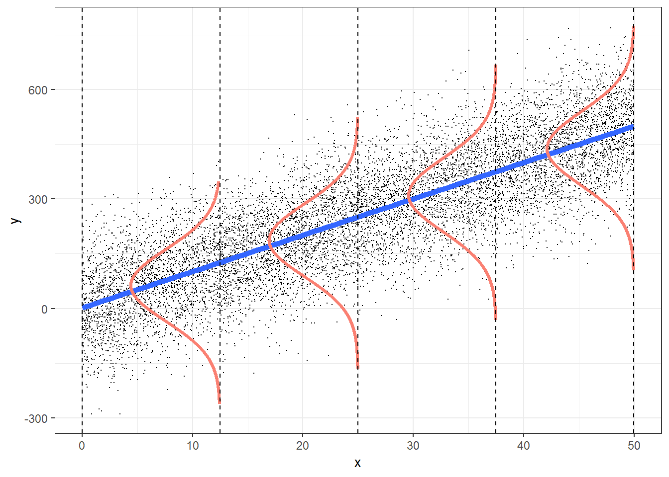
FIGURE 14.1: Figure illustrating the simple linear regression model. From https://bookdown.org/roback/bookdown-bysh/
14.2 Generalized linear models
14.2.1 Nomenclature
One thing that is sometimes confusing is the difference between General Linear Models and Generalized Linear Models. The term General Linear Model is used to acknowledge that several statistical methods, listed below, can all be viewed as fitting a linear model with the same underlying assumptions (linearity, constant variance, normal residuals, and independence):
- a t-test is a linear model with a single categorical predictor with 2 levels
- ANOVA is a linear model with a single categorical predictor with \(\ge 2\) levels
- ANCOVA is a linear model containing a continuous predictor and a categorical predictor, but no interaction between the two (thus, the different groups have a common slope)
- more general models may contain a mix of continuous and categorical variables and possible interactions between variables
Generalized linear models, by contrast, refers to a broader class of models that allow for alternative probability distributions in addition to the Normal distribution. Historically, the development of generalized linear models focused on statistical distributions in the exponential family (McCullagh & Nelder, 1989), which includes the normal distribution with constant variance, Poisson, Binomial, Gamma, among others. These distributions can all be written in a specific form (eq. (14.2)), which facilitated the development of common methods for model fitting and a unified theory for interpreting model parameters (McCulloch & Neuhaus, 2005):
\[\begin{equation} f(y | \theta, \tau) = h(y, \tau)\exp\Big(\frac{b(\theta)T(y)-A(\theta)}{d(\tau)}\Big) \tag{14.2} \end{equation}\]
If you were to take a class on generalized linear models in a statistics department, you would likely be required to show that various statistical distributions (e.g., those listed above) can be written in this form. You might also learn how derive the mean and variance of each distribution from this general expression (see e.g., Table 2.1 from McCullagh & Nelder, 1989; Section 8.7 of Zuur et al., 2009). The fact that it is possible to derive general results for distributions in the exponential family is really quite cool! At the same time, you do not need to work through those exercises to be able to use generalized linear models to analyze your data. Further, it is relatively easy to extend the basic conceptual approach (constructing models where we express parameters of common statistical distributions as a function of predictor variables) to allow for a much richer class of models - i.e., there is no need to limit oneself to distributions from the exponential family.
14.3 Describing the data generating mechanism
With distributions other than the Normal distribution, we will no longer be able to write our models in terms of a “signal + error”. Yet, it may still be conceptually useful to consider how these models capture systematic and random variation in the data. Systematic variation is captured by modeling some transformation of the mean, \(g(\mu_i)\), as a linear function of predictor variables. In addition, we will assume that the response \(Y_i|X_i\) comes from a particular statistical distribution.
Systematic component:
- \(\eta_i = g(\mu_i) = \beta_0 + \beta_1X_{1,i} + \ldots \beta_pX_{p,i}\); \(g( )\) is called the link function; \(\eta_i\) is called the linear predictor.
- \(\Rightarrow E[Y_i|X_i] = \mu_i = g^{-1}(\beta_0 + \beta_1X_{1,i} + \ldots \beta_pX_{p,i})\); \(g^{-1}()\) is the inverse link function.
Random component:
- We write \(Y_i|X_i \sim f(y_i|x_i), i=1, \ldots, n\)
- \(f(y_i|x_i)\) is a probability density or probability mass function of a statistical distribution and describes unmodeled variation about \(\mu_i = E[Y_i|X_i]\)
Examples of generalized linear models are given below.
Linear Regression:
- \(f(y_i|x_i) = N(\mu_i, \sigma^2)\)
- \(E[Y_i|X_i]= \mu_i = \beta_0 + \beta_1X_1 + \ldots \beta_pX_p\)
- \(g(\mu_i) = \mu_i\), the identity link
- \(\mu_i = g^{-1}(\eta_i) = \eta_i= \beta_0 + \beta_1X_{1,i} + \ldots \beta_pX_{p,i}\)
Poisson regression:
- \(f(y_i|x_i) \sim Poisson(\lambda_i)\)
- \(E[Y_i|X_i] = \mu_i = \lambda_i\)
- \(g(\mu_i) = \eta_i = log(\lambda_i) = \beta_0 + \beta_1X_{1,i} + \ldots \beta_pX_{p,i}\)
- \(\mu_i = g^{-1}(\eta_i) = exp(\eta_i) = exp(\beta_0 + \beta_1X_{1,i} + \ldots \beta_pX_{p,i})\)
Logistic regression:
- \(f(y_i|x_i) \sim\) Bernoulli\((p_i)\)
- \(E[Y_i|X_i] = p_i\)
- \(g(\mu_i) = \eta_i = \text{logit}(p_i) = \log(\frac{p_i}{1-p_i}) = \beta_0 + \beta_1X_{1,i} + \ldots \beta_pX_{p,i}\)
- \(\mu_i = g^{-1}(\eta_i) = \Large \frac{\exp^{\eta_i}}{1+\exp^{\eta_i}} = \frac{\exp^{\beta_0 + \beta_1X_{1,i} + \ldots \beta_pX_{p,i}}}{1+\exp^{\beta_0 + \beta_1X_{1,i} + \ldots \beta_pX_{p,i}}}\)
14.3.1 Link functions, \(g()\)
Link functions allow the “systematic component” (\(\beta_0 + \beta_1X_1 + \ldots \beta_pX_p\)) to live on \((-\infty, \infty)\) while keeping the \(\mu_i\) consistent with the range of the response variable. For example, \(g^-1(\eta) = exp(\eta)\) ensures that the mean in Poisson regression models, \(\lambda_i\), is greater than or equal to 0. Similarly, \(g^{-1}(\eta) = \Large \frac{exp(\eta)}{1+ exp(\eta)}\) ensures the mean of logistic regression models, \(p_i\), is between 0 and 1 (Figure 14.2):
eta<-seq(-10,10, length=1000)
mean.Poisson<-exp(eta)
mean.Logistic<-exp(eta)/(1+exp(eta))
pdat<-data.frame(eta, mean.Poisson, mean.Logistic)
p1<-ggplot(pdat,aes(eta, mean.Poisson))+geom_line()+
  xlab(expression(eta))+ylab(expression(exp(eta)))+ggtitle("Poisson Regression")
p2<-ggplot(pdat,aes(eta, mean.Logistic))+geom_line()+
  xlab(expression(eta))+ylab(expression(exp(eta)/(1+exp(eta))))+
  ggtitle("Logistic Regression")
gridExtra::grid.arrange(p1, p2, nrow=1)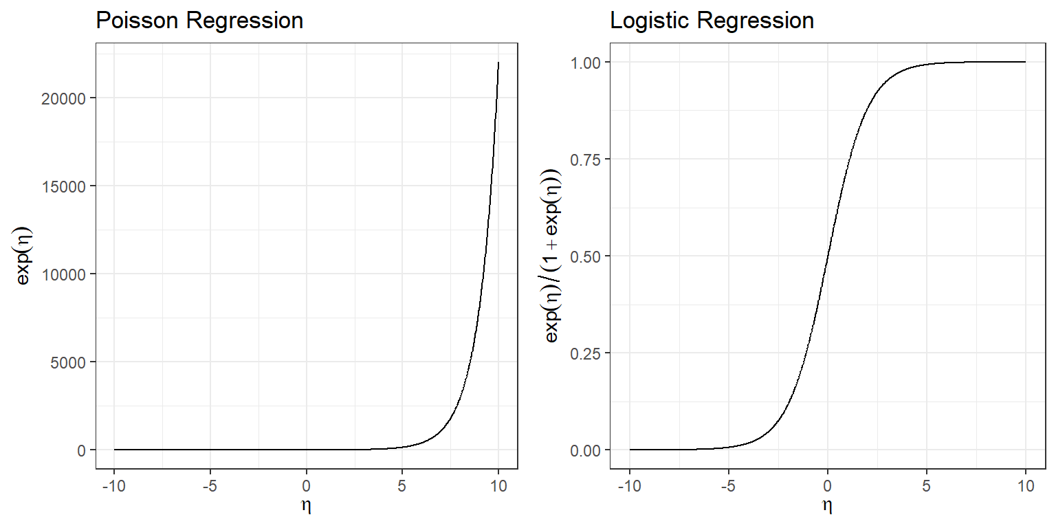
FIGURE 14.2: Mean response versus linear predictor for Poisson and Logistic regression models.
Poisson Regression:
- \(g(\mu_i) = \eta_i = log(\lambda_i) = \beta_0 + \beta_1x_1 + \ldots \beta_px_p\), range = \((-\infty, \infty)\)
- \(\Rightarrow \mu_i = exp(\beta_0 + \beta_1x_1 + \ldots \beta_px_p)\) has range = \([0, \infty]\)
Logistic regression:
- \(g(\mu_i) = \eta_i = log(\frac{p_i}{1-p_i}) = \beta_0 + \beta_1x_1 + \ldots \beta_px_p\), range = \((-\infty, \infty)\)
- \(\mu_i = g^{-1}(\eta_i) = \frac{\exp^{\eta_i}}{1+\exp^{\eta_i}} = \frac{\exp^{\beta_0 + \beta_1x_1 + \ldots \beta_px_p}}{1+\exp^{\beta_0 + \beta_1x_1 + \ldots \beta_px_p}}\), range = \((0, 1)\)
Now that we have defined terms and seen how these definitions apply to specific distributions, let’s consider a hypothetical example using the Poisson regression.
14.4 Example: Poisson regression for pheasant counts
Consider a wildlife researcher that is interested in modeling how pheasant abundance varies with the amount of grassland cover. She divides the landscape up into a series of plots. She and several colleagues walk transects in these plots with their hunting dogs to location and flush pheasants, leading to a count in each plot, \(y_i\). They also use a Geographic Information System to capture the % grassland cover in each plot, \(x_i\).

FIGURE 14.3: Picture of a pheasant by Gary Noon - Flickr, CC BY-SA 2.0.
We could fit a Poisson regression model (we will see how to do this in R in the next Section) in which the mean count depends on grassland abundance. To describe the model using equations, we would write:
- \(Y_i|X_i \sim Poisson(\lambda_i)\)
- \(log(\lambda_i) = \beta_0 + \beta_1X_{i}\)
Because the mean of the Poisson distribution is \(\lambda\), we have assumed:
- \(E[Y_i|X_i] = \lambda_i = g^{-1}(\beta_0 + \beta_1X_{i}) = \exp(\beta_0 + \beta_1X_{1,i})\)
In English, we model the log of the mean as a linear function of grassland abundance (this is the systematic component of the model). Further, we assume the observed counts, \(Y_1, Y_2, \ldots, Y_n\), are independent Poisson random variables, with means that depend on the amount of grassland cover (\(X_i\)) (this is the random component).
14.4.1 Poisson regression assumptions
These next two subsections were slightly modified from the online version of Roback & Legler (2021), which is licensed under Creative Commons Attribution-NonCommercial-ShareAlike 4.0 International License.
Much like linear regression, we can list the underlying assumptions of Poisson regression:
- Poisson Response: The response variable is a count per unit of time or space, described by a Poisson distribution.
- Independence: The observations must be independent of one another.
- Mean=Variance: By definition, the mean of a Poisson random variable must be equal to its variance.
- Linearity: The log of the mean rate, log(\(\lambda\)), must be a linear function of x.
Figure 14.4 illustrates a comparison of linear regression and Poisson regression.
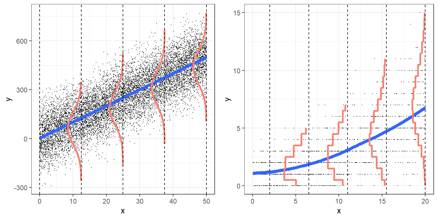
FIGURE 14.4: Regession Models: Linear Regression (left) and Poisson Regression (right)
- For the linear regression model (left panel of Fig. 14.4), the responses appear to be approximately normal for any given value of \(X\). For the Poisson regression model (right panel of Fig. 14.4), the responses follow a Poisson distribution for any given value of \(X\). For Poisson regression, small values of \(\lambda\) are associated with a distribution that is noticeably skewed with lots of small values and only a few larger ones. As \(\lambda\) increases the distribution of the responses begins to look more and more like a normal distribution.
- In the linear regression model, the variation in \(Y\) at each level of X, \(\sigma^2\), is the same. For Poisson regression, the variance increases with the mean (remember, the variance is equal to the mean for the Poisson distribution).
- In the case of linear regression, the mean responses for each level of \(X\) falls on a line, \(E[Y_i|X_i] = \mu_i = \beta_0+\beta_1X_i\). In the case of the Poisson model, the mean values of \(Y\) at each level of \(X\) fall on the curve \(\lambda_i = \exp(\beta_0+\beta_1X_i)\).