Chapter 8 Modeling Strategies
Learning objectives
Gain an appreciation for challenges associated with selecting among competing models and performing multi-model inference.
Understand common approaches used to select a model (e.g., stepwise selection using p-values, AIC, Adjusted \(R^2\)).
Understand the implications of model selection for statistical inference.
Gain exposure to alternatives to traditional model selection, including full model inference (df spending), model averaging, and penalized likelihood/regularization techniques.
Be able to evaluate evaluate model performance using cross-validation and model stability using the bootstrap.
Be able to choose an appropriate modeling strategy, depending on the goal of the analysis (describe, predict, or infer).
8.1 Goals of multivariable regression modeling
Before deciding on an appropriate modeling strategy, it is important to recognize that there are multiple possible objectives motivating the need for a model (Shmueli, 2010; Kuiper & Sklar, 2012; Tredennick, Hooker, Ellner, & Adler, 2021). Kuiper & Sklar (2012) lists 3 general modeling objectives, to describe, predict, or explain, which closely mimics the goals outlined by Tredennick et al. (2021), exploration, prediction, and inference.
Describe: we may just want to capture the main patterns in the data in a parsimonious way. This may be a first step in trying to understand which factors are related to the response variable. Note, describing associations between variables is a much less lofty goal than evaluating cause and effect.
Predict: we may want to use data we have in hand to make predictions about future data. Here, we may not need to worry about causality and confounding (capturing associations may be just fine). We may be able to predict the average life expectancy for a country based on tvs per capita (Figure 7.1) or the number of severe sunburns from local ice creme sales (Figure 7.3). Yet these predictions do not capture causal mechanisms, and thus, we will often find that our model fails to predict when we try to apply it to a new situation where the underlying correlations among our predictor variables differs from the correlations among predictors in the data set we used to fit the model.
Explain/Infer: we may have a biological hypothesis or set of competing hypotheses about how the world works. These hypotheses might suggest that certain variables, or combination of variables, are causally related to the response variable. When trying to infer causal relationships between predictor and response variables, we have to think more broadly about links among our observed predictor variables (not just links between predictors and the response). In addition, we must consider possible confounding by unmeasured or omitted variables. Essentially, we need to keep in mind everything from Section 7.
Clearly, the least lofty goal is to explore or describe patterns, but whether one views prediction or inference as the most challenging or lofty goal may depend on whether predictions are expected to match observations in novel situations or just under conditions similar to those used to train the model. If we want to be able to predict what will happen when the system changes, we will need to have a strong understanding of mechanisms driving observed patterns.
It is important to consider your goals when deciding upon a modeling strategy (Table 8.1, recreated Table 2 from Tredennick et al., 2021). I collaborate mainly with scientists that work with observational data. Often, they express their questions in broad terms, such as, “I want to know which predictor variables are most important.” When pressed, they may indicate they are interested a bit in all of the above (describing patterns, explaining patterns, and predicting patterns). The main challenge to “doing all of the above” is that it is all too easy to detect patterns in data that do not represent causal mechanisms, leading to models that fail to predict new data well. This can result in a tremendous waste of money and resources. We need to consider the impact of applying an overly flexible modeling strategy if our goal is to identify important associations among variables (explain) or if our goal is to develop a predictive model (predict). I learned of the dangers of overfitting the hard way while getting my Masters degree in Biostatistics at the University of North Carolina-Chapel Hill (see Section 8.2).
| Parameter | Exploration | Inference | Prediction |
|---|---|---|---|
| Purpose | generate hypotheses | test hypotheses | forecast the future accurately |
| Priority | thoroughness | avoid false positives | minimize error |
| A priori hypothesis | not necessary | essential | not necessary, but may inform model specification |
| Emphasis on model selection | important | minimal | important |
| Key statistical tools | any | null hypothesis significance tests | AIC; regularization; machine learning; cross-validation; out-of-sample validation |
| Pitfalls | fooling yourself with overfitted models with spurious covariate effects | misrepresenting exploratory tests as tests of a priori hypotheses | failure to rigorously validate prediction accuracy with independent data |
If we have competing models for how the world works (e.g., different causal networks; Section 7), then we can formulate mechanistic models that represent these competing hypotheses. In some cases you may have to write our own code to fit models using Maximum Likelihood (Section 10) and Bayesian machinery (Section 11); we will be learning about these methods soon. We can then compare predictions from these models or evaluate their ability to match qualitative patterns in data (“goodness-of-fit”), ideally across multiple study systems, to determine if our theories hold up to the scrutiny of data. If you find yourself in this situation (i.e., doing inference), consider yourself lucky (or good); you are doing exciting science.
8.2 My experience
In the first year of my Masters degree, I took a Linear Models class from Dr. Keith Muller. For our mid-term exam, we were given a real data set and asked to develop a model for patients’ Serum Albumin levels32. The data set contained numerous predictors, some with missing data. We were given a weekend to complete the analysis and write up a report on our findings. Importantly, we were instructed to take one of two approaches:
If we knew the subject area (or, could quickly get up speed), then we could choose to test a set of a priori hypotheses regarding whether specific explanatory variables were associated with Serum Albumin levels. We were encouraged to consider potential issues related to multiple comparisons and to adjust our \(\alpha\) level to ensure a overall type I error rate of less than 5%33.
Split the data into a “training” data set (with 80% of the original observations) and a “test” data set (with the remaining 20% of the observations). Use the training data set to determine an appropriate model. Then, evaluate the model’s performance using the test data set. When determining an appropriate model, we were instructed to use various residual and diagnostic plots and to also consider the impact of that an overly data-driven or flexible modeling approach might have on future model performance.
I don’t think anyone from our class knew anything about blood chemistry or kidney failure, so I suspect everyone went with option 2. A few things I recall from my approach and the final outcome:
I grouped variables into similar categories (e.g., socio-economic status, stature [height, weight, etc], dietary intake variables) and examined variables within each group for collinearity. I then picked a single “best” variable in each category using simple linear regressions (i.e., fitting models with a single predictor to determine which variable was most highly correlated with the response).
I fit a model that combined the “best” variables from each category and evaluated model assumptions (Normality, constant variance, linearity). Residual plots all looked good - no major assumption violations.
I allowed for a non-linear effect of weight using a quadratic polynomial (see Section 4.2). To be honest, I cannot remember why. The decision, however, was likely arrived at after looking at the data and noticing a trend in the residuals or finding that a quadratic term was highly significant when included in the model.
I applied various stepwise regression methods (see Section 8.3.1) and always arrived at the same reduced model.
I looked to see if I might have left off any important variables by adding them to this reduced model arrived at in step [4]. None of the added variables were statistically significant. This step gave me further confidence that I had found the best model for the job.
Lastly, I again looked at residual diagnostics associated with the reduced model. Everything looked hunky-dory.
I remember being highly confident that I found THE BEST model and that the assumptions were all reasonable. Looking back, I recalled that my model had an \(R^2\) of close to 90%. When I began teaching, I went back and found my actual test. The initial \(R^2\) was only 28%! Then came the moment of truth. I evaluated the model’s performance using the test data. My model only explained 7.6% of the variability (Figure 8.1)! I had a hard time believing it. Many other students had similar experiences. I had learned an important lesson that would stick with me for the rest of my professional life. It is way to easy to detect a signal in noise if you allow for too flexible of a modeling approach.
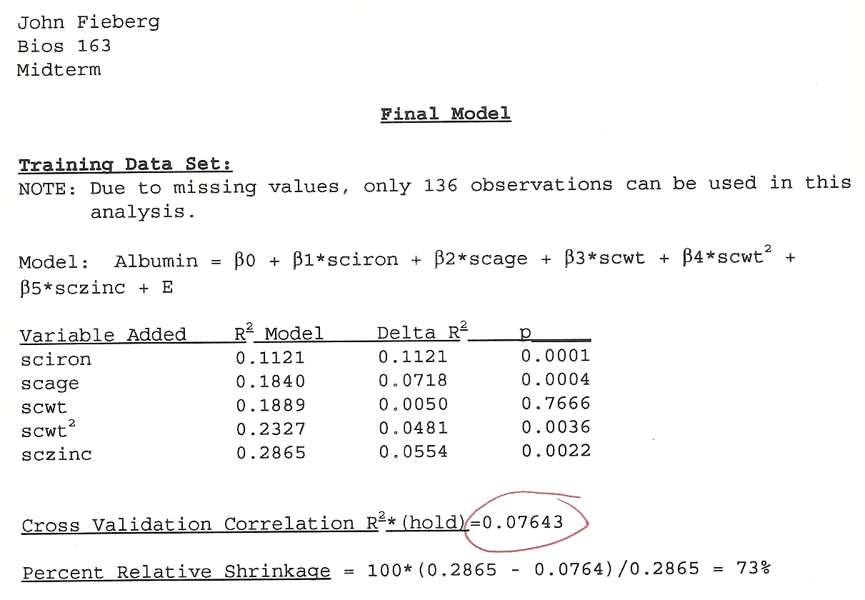
FIGURE 8.1: My mid-tem exam from my Linear Models class.
8.3 Stepwise Algorithms
There are many ways to sift through model space to determine a set of predictors that are most highly associated with a response variable. At the extreme, one can specify a set of predictors and then fit “all possible models” that include 1 or more of these predictors along with a null model containing only an intercept (e.g., using the dredge function in the MuMIn package; Barton, 2020). Having fit all possible models, one must specify a criterion for choosing a “best model.” For linear models, one could use to use the adjusted-\(R^2\) (Section 3.3). Alternatively, one could choose to use one of a number of various information criterion (e.g., AIC, BIC, WAIC, DIC). The Akaike information criterion, AIC (Akaike, 1974), is probably the most well known and most frequently used information criterion:
\[AIC = -2\log l(\hat{\theta}) + 2p\] where \(\log l\) is the likelihood of the data evaluated at the estimated parameter values, \(\hat{\theta}\) and provides a measure of model fit and \(p\) is the number of parameters in the model (Section 10). The likelihood will always increase as we add more parameters, but AIC may not due to the penalty, \(2p\). Simpler models with smaller values of AIC are preferred, all else being equal.
Alternatively, one can try to successfully build bigger and better models (by adding 1 variable at a time), referred to as forward-stepwise selection, or try to build slimmer and better models (by eliminating 1 variable at a time from an initial full model), referred to as backwards elimination. Either approach will result in many comparisons of nested models; two models are nested if you can get from the more complex model to the simpler model by by setting one or more parameters = 0. As one example, the following two models are nested:
- \(\mbox{Sleep} = \beta_0 + \beta_1\mbox{Danger} + \beta_2\mbox{LifeSpan}\)
- \(\mbox{Sleep} = \beta_0 + \beta_1\mbox{Danger}\)
whereas the two models below are not:
- \(\mbox{Sleep} = \beta_0 + \beta_1\mbox{Danger}\)
- \(\mbox{Sleep} = \beta_0 + \beta_1\mbox{Lifespan}\)
For nested models, we can use p-values from t-tests, F-tests, or likelihood-ratio tests to compare models (in addition to AIC or adjusted-\(R^2\)). In the next section, we will briefly consider stepwise selection algorithms using AIC.
8.3.1 Backwards elimination and forward-stepwise selection
To apply backwards stepwise selection, we:
- Fit a full model containing all predictors of interest.
- Consider all possible models formed by dropping 1 of these predictors
- Keep the current model, or drop the “worst” predictor depending on:
- p-values from the individual t-tests (drop the variable with the highest p-value, if \(>0.05\))
- Adjusted \(R^2\) values (higher values are better)
- AIC (lower values are better)
- Rinse and repeat until you can no longer improve the model
The stepAIC function in the MASS library will do this for us. Let’s explore this approach using the mammal sleep data set from Section 6. Before we begin, it is important to recognize that this data set has many missing values for several of the variables. This can create issues when compare models since R will by default drop any observations where one or more of the variables are missing. Thus, the number observations will change depending on which predictors are included in the model, making comparisons using AIC or adjusted \(R^2\) problematic. Ideally, we would consider a multiple imputation strategy to deal with this issue, but for now, we will just consider the data set with complete observations
library(openintro)
library(dplyr)
data(mammals, package="openintro")
mammalsc<-mammals %>% filter(complete.cases(.))
MASS::stepAIC(lm(total_sleep ~ life_span + gestation + log(brain_wt) +
                     log(body_wt) + predation + exposure + danger, data=mammalsc))
## Start: AIC=100.44
## total_sleep ~ life_span + gestation + log(brain_wt) + log(body_wt) +
## predation + exposure + danger
##
## Df Sum of Sq RSS AIC
## - log(body_wt) 1 0.412 313.99 98.491
## - life_span 1 1.218 314.79 98.598
## - log(brain_wt) 1 12.516 326.09 100.079
## - gestation 1 13.389 326.96 100.192
## <none> 313.58 100.436
## - exposure 1 18.527 332.10 100.847
## - predation 1 31.079 344.65 102.405
## - danger 1 92.636 406.21 109.307
##
## Step: AIC=98.49
## total_sleep ~ life_span + gestation + log(brain_wt) + predation +
## exposure + danger
##
## Df Sum of Sq RSS AIC
## - life_span 1 0.977 314.96 96.621
## - gestation 1 13.113 327.10 98.209
## <none> 313.99 98.491
## - exposure 1 19.446 333.43 99.014
## - predation 1 30.876 344.86 100.430
## - log(brain_wt) 1 31.497 345.48 100.506
## - danger 1 92.380 406.37 107.323
##
## Step: AIC=96.62
## total_sleep ~ gestation + log(brain_wt) + predation + exposure +
## danger
##
## Df Sum of Sq RSS AIC
## - gestation 1 12.206 327.17 96.218
## <none> 314.96 96.621
## - exposure 1 18.987 333.95 97.080
## - predation 1 30.083 345.05 98.453
## - log(brain_wt) 1 34.465 349.43 98.983
## - danger 1 92.153 407.12 105.400
##
## Step: AIC=96.22
## total_sleep ~ log(brain_wt) + predation + exposure + danger
##
## Df Sum of Sq RSS AIC
## <none> 327.17 96.218
## - exposure 1 16.239 343.41 96.253
## - predation 1 41.155 368.32 99.194
## - log(brain_wt) 1 90.786 417.96 104.504
## - danger 1 108.584 435.75 106.255##
## Call:
## lm(formula = total_sleep ~ log(brain_wt) + predation + exposure +
## danger, data = mammalsc)
##
## Coefficients:
## (Intercept) log(brain_wt) predation exposure danger
## 16.5878 -0.8800 2.2321 0.9066 -4.5425We see a set of tables comparing the current “best” model (<none> indicating no variables have been dropped) to all possible models that have 1 fewer predictor, sorted from lowest (best fitting) to highest (worst fitting) as judged by AIC. For example, in the first table, we see that dropping any of (log(body_wt), life_span, log(brain_wt), gestation) will result in a model with a lower AIC than the one keeping all variables. On the other hand, dropping any of (exposure, predation, or danger) will result in a model with a worse AIC than the one keeping all variables. At this step, we drop log(body_wt) since dropping it results in a model with the lowest AIC (98.491) among all 6-variable models. We repeat the algorithm, dropping lifespan, and then once more, dropping gestation. At that point, dropping any of (log(brain_wt), predation, exposure, danger) will result in a model that has a higher AIC, so we stop.
Forward stepwise selection moves in the opposite direction and can be implemented using the step function:
min.model <- lm(total_sleep ~ 1, data=mammalsc)
step(min.model, scope=( ~ life_span + gestation + log(brain_wt) + log(body_wt) +
                          predation + exposure + danger),
                          direction="forward", data=mammalsc)
## Start: AIC=131.15
## total_sleep ~ 1
##
## Df Sum of Sq RSS AIC
## + log(brain_wt) 1 352.15 557.17 112.58
## + exposure 1 351.08 558.25 112.66
## + log(body_wt) 1 346.71 562.62 112.99
## + gestation 1 343.34 565.98 113.24
## + danger 1 332.07 577.25 114.07
## + predation 1 148.94 760.38 125.64
## + life_span 1 133.00 776.32 126.51
## <none> 909.32 131.15
##
## Step: AIC=112.58
## total_sleep ~ log(brain_wt)
##
## Df Sum of Sq RSS AIC
## + danger 1 179.991 377.18 98.192
## + predation 1 118.745 438.43 104.512
## + exposure 1 83.765 473.41 107.736
## + gestation 1 38.295 518.88 111.588
## <none> 557.17 112.579
## + life_span 1 11.296 545.88 113.718
## + log(body_wt) 1 6.190 550.98 114.109
##
## Step: AIC=98.19
## total_sleep ~ log(brain_wt) + danger
##
## Df Sum of Sq RSS AIC
## + predation 1 33.773 343.41 96.253
## + gestation 1 19.139 358.04 98.005
## <none> 377.18 98.192
## + exposure 1 8.857 368.32 99.194
## + life_span 1 0.519 376.66 100.135
## + log(body_wt) 1 0.354 376.83 100.153
##
## Step: AIC=96.25
## total_sleep ~ log(brain_wt) + danger + predation
##
## Df Sum of Sq RSS AIC
## + exposure 1 16.2392 327.17 96.218
## <none> 343.41 96.253
## + gestation 1 9.4578 333.95 97.080
## + log(body_wt) 1 0.6927 342.72 98.168
## + life_span 1 0.0103 343.40 98.251
##
## Step: AIC=96.22
## total_sleep ~ log(brain_wt) + danger + predation + exposure
##
## Df Sum of Sq RSS AIC
## <none> 327.17 96.218
## + gestation 1 12.2056 314.96 96.621
## + log(body_wt) 1 0.0943 327.08 98.206
## + life_span 1 0.0696 327.10 98.209##
## Call:
## lm(formula = total_sleep ~ log(brain_wt) + danger + predation +
## exposure, data = mammalsc)
##
## Coefficients:
## (Intercept) log(brain_wt) danger predation exposure
## 16.5878 -0.8800 -4.5425 2.2321 0.9066In this case, we end up at the same place. This may seem reassuring as it tells us that we arrive at the same “best model” regardless of which approach we choose. Yet, what really matters is how these algorithms perform across multiple data sets (see Section 8.7.2). Therein lies many problems. As noted by Frank Harrell in his Regression Modeling Strategies book (Harrell Jr, 2015), with stepwise selection:
- \(R^2\) values are biased high.
- The ordinary F and \(\chi^2\) test statistics used to test hypotheses do not have the claimed distribution
- SEs of regression coefficients will be biased low and confidence intervals will be falsely narrow.
- p-values will be too small and do not have the proper meaning (due to multiple comparison problems).
- Regression coefficients will be biased high in absolute magnitude.
- Rather than solve problems caused by collinearity, variable selection is made arbitrary by collinearity.
- It allows us not to think about the problem.
Issues with p-values are rather easy to understand in the context of multiple comparisons and multiple testing, whereas the bias in regression coefficients may be more surprising to some readers. To understand why regression coefficient estimators will be biased high, it is important to recognize that inclusion in the final model depends not on the true relationship between the explanatory and response variables but rather on the estimated relationship determined from the original sample. A variable is more likely to be included if by chance its importance in the original sample was overestimated than if it was underestimated (Copas & Long, 1991). These issues are more pronounced when applied to small data sets with lots of predictors; stepwise selection methods can easily select noise variables rather than ones that are truly important.
Issues with stepwise selection are well known to statisticians, who agree that these methods should be abandoned (Anderson & Burnham, 2004; Whittingham, Stephens, Bradbury, & Freckleton, 2006; Hegyi & Garamszegi, 2011; Giudice, Fieberg, & Lenarz, 2012; Fieberg & Johnson, 2015). Yet, they are still routinely used, likely because they appear to be objective and “let the data speak” rather than forcing the analyst to think. Stepwise selection methods can sometimes be useful for identifying important associations, but any results should be treated cautiously. I.e., it is best to consider these methods as useful for generating new hypotheses; these hypotheses should be tested with new, independent data.
If you are not convinced, try this simple simulation example posted by Florian Hartig here:
set.seed(1)
library(MASS)

# Generate 200 observations with 100 predictors that are unrelated to the response variable
dat <- data.frame(matrix(runif(20000), ncol = 100))
dat$y <- rnorm(200)

# Fit a full model containing all predictors and test for significance.
fullModel <- lm(y ~ . , data = dat)
summary(fullModel)
##
## Call:
## lm(formula = y ~ ., data = dat)
##
## Residuals:
## Min 1Q Median 3Q Max
## -1.95280 -0.39983 -0.01572 0.46104 1.61967
##
## Coefficients:
## Estimate Std. Error t value Pr(>|t|)
## (Intercept) 2.19356 1.44518 1.518 0.1322
## X1 0.58079 0.32689 1.777 0.0787 .
## X2 -0.52687 0.32701 -1.611 0.1103
## X3 0.27721 0.33117 0.837 0.4046
## X4 -0.18342 0.30443 -0.602 0.5482
## X5 -0.18544 0.29011 -0.639 0.5242
## X6 -0.18382 0.31406 -0.585 0.5597
## X7 -0.46290 0.28349 -1.633 0.1057
## X8 -0.21527 0.29856 -0.721 0.4726
## X9 0.12216 0.30359 0.402 0.6883
## X10 -0.02594 0.33828 -0.077 0.9390
## X11 0.25669 0.29482 0.871 0.3860
## X12 -0.10183 0.30164 -0.338 0.7364
## X13 0.49507 0.33438 1.481 0.1419
## X14 0.16642 0.33659 0.494 0.6221
## X15 0.11402 0.32964 0.346 0.7302
## X16 -0.17640 0.31619 -0.558 0.5782
## X17 -0.03129 0.31830 -0.098 0.9219
## X18 -0.28201 0.29681 -0.950 0.3444
## X19 0.02209 0.29664 0.074 0.9408
## X20 0.25063 0.29855 0.839 0.4032
## X21 -0.02479 0.30556 -0.081 0.9355
## X22 -0.01187 0.31265 -0.038 0.9698
## X23 -0.58731 0.31491 -1.865 0.0651 .
## X24 -0.27343 0.32894 -0.831 0.4078
## X25 -0.22745 0.29223 -0.778 0.4382
## X26 0.18606 0.35755 0.520 0.6040
## X27 -0.26998 0.33302 -0.811 0.4195
## X28 0.09683 0.32235 0.300 0.7645
## X29 0.36746 0.32915 1.116 0.2670
## X30 -0.26027 0.31335 -0.831 0.4082
## X31 -0.07890 0.28822 -0.274 0.7849
## X32 -0.07879 0.32662 -0.241 0.8099
## X33 -0.27736 0.34542 -0.803 0.4239
## X34 -0.21118 0.34514 -0.612 0.5420
## X35 0.17595 0.30706 0.573 0.5679
## X36 0.17084 0.30423 0.562 0.5757
## X37 0.28246 0.29520 0.957 0.3410
## X38 0.01765 0.32873 0.054 0.9573
## X39 0.07598 0.27484 0.276 0.7828
## X40 0.09714 0.34733 0.280 0.7803
## X41 -0.16985 0.31608 -0.537 0.5922
## X42 -0.25184 0.33203 -0.758 0.4500
## X43 -0.08306 0.29306 -0.283 0.7774
## X44 -0.17389 0.31090 -0.559 0.5772
## X45 -0.30756 0.30995 -0.992 0.3235
## X46 0.61520 0.30961 1.987 0.0497 *
## X47 -0.61994 0.32461 -1.910 0.0591 .
## X48 0.62326 0.33822 1.843 0.0684 .
## X49 0.35504 0.30382 1.169 0.2454
## X50 0.09683 0.31925 0.303 0.7623
## X51 0.17292 0.30770 0.562 0.5754
## X52 -0.06560 0.30549 -0.215 0.8304
## X53 -0.29953 0.32318 -0.927 0.3563
## X54 0.06888 0.32289 0.213 0.8315
## X55 0.05695 0.32103 0.177 0.8596
## X56 0.26284 0.32914 0.799 0.4265
## X57 0.10457 0.29788 0.351 0.7263
## X58 -0.19239 0.30729 -0.626 0.5327
## X59 0.02371 0.29171 0.081 0.9354
## X60 -0.12842 0.32321 -0.397 0.6920
## X61 0.06931 0.30015 0.231 0.8179
## X62 -0.27227 0.31918 -0.853 0.3957
## X63 -0.17359 0.32287 -0.538 0.5920
## X64 -0.41846 0.33808 -1.238 0.2187
## X65 -0.37243 0.31872 -1.169 0.2454
## X66 0.36263 0.33034 1.098 0.2750
## X67 -0.10120 0.30663 -0.330 0.7421
## X68 -0.33790 0.33633 -1.005 0.3175
## X69 -0.05326 0.30171 -0.177 0.8602
## X70 -0.01047 0.33111 -0.032 0.9748
## X71 -0.46896 0.32387 -1.448 0.1508
## X72 -0.29867 0.33543 -0.890 0.3754
## X73 -0.32556 0.33183 -0.981 0.3289
## X74 0.21187 0.31690 0.669 0.5053
## X75 0.63659 0.31144 2.044 0.0436 *
## X76 0.13838 0.31642 0.437 0.6628
## X77 -0.18846 0.29382 -0.641 0.5227
## X78 0.06325 0.29180 0.217 0.8289
## X79 0.07256 0.30145 0.241 0.8103
## X80 0.33483 0.34426 0.973 0.3331
## X81 -0.33944 0.35373 -0.960 0.3396
## X82 -0.01291 0.32483 -0.040 0.9684
## X83 -0.06540 0.27637 -0.237 0.8134
## X84 0.11543 0.32813 0.352 0.7257
## X85 -0.20415 0.31476 -0.649 0.5181
## X86 0.04202 0.33588 0.125 0.9007
## X87 -0.33265 0.29159 -1.141 0.2567
## X88 -0.49522 0.31251 -1.585 0.1162
## X89 -0.39293 0.33358 -1.178 0.2417
## X90 -0.34512 0.31892 -1.082 0.2818
## X91 0.10540 0.28191 0.374 0.7093
## X92 -0.08630 0.30297 -0.285 0.7764
## X93 0.02402 0.32907 0.073 0.9420
## X94 0.51255 0.32139 1.595 0.1139
## X95 -0.19971 0.30634 -0.652 0.5160
## X96 -0.09592 0.34585 -0.277 0.7821
## X97 -0.18862 0.29266 -0.644 0.5207
## X98 0.14997 0.34858 0.430 0.6680
## X99 -0.08061 0.30400 -0.265 0.7914
## X100 -0.34988 0.31664 -1.105 0.2718
## ---
## Signif. codes: 0 '***' 0.001 '**' 0.01 '*' 0.05 '.' 0.1 ' ' 1
##
## Residual standard error: 0.9059 on 99 degrees of freedom
## Multiple R-squared: 0.4387, Adjusted R-squared: -0.1282
## F-statistic: 0.7739 on 100 and 99 DF, p-value: 0.8987# Perform model selection using AIC and then summarize the results
selection <- stepAIC(fullModel, trace=0)
summary(selection)##
## Call:
## lm(formula = y ~ X1 + X2 + X3 + X5 + X7 + X13 + X20 + X23 + X30 +
## X37 + X42 + X45 + X46 + X47 + X48 + X64 + X65 + X66 + X71 +
## X75 + X80 + X81 + X87 + X88 + X89 + X90 + X94 + X100, data = dat)
##
## Residuals:
## Min 1Q Median 3Q Max
## -2.04660 -0.50885 0.05722 0.49612 1.53704
##
## Coefficients:
## Estimate Std. Error t value Pr(>|t|)
## (Intercept) 1.0314 0.5045 2.044 0.04244 *
## X1 0.4728 0.2185 2.164 0.03187 *
## X2 -0.3809 0.2012 -1.893 0.06008 .
## X3 0.3954 0.1973 2.004 0.04668 *
## X5 -0.2742 0.1861 -1.473 0.14251
## X7 -0.4442 0.1945 -2.284 0.02359 *
## X13 0.4396 0.1980 2.220 0.02775 *
## X20 0.3984 0.1918 2.078 0.03924 *
## X23 -0.4137 0.2081 -1.988 0.04836 *
## X30 -0.3750 0.1991 -1.884 0.06125 .
## X37 0.4006 0.1989 2.015 0.04550 *
## X42 -0.3934 0.2021 -1.946 0.05325 .
## X45 -0.3197 0.2063 -1.550 0.12296
## X46 0.3673 0.1992 1.844 0.06690 .
## X47 -0.4240 0.2029 -2.090 0.03811 *
## X48 0.5130 0.1937 2.649 0.00884 **
## X64 -0.3676 0.2094 -1.755 0.08102 .
## X65 -0.2887 0.1975 -1.462 0.14561
## X66 0.2769 0.2107 1.315 0.19039
## X71 -0.5301 0.2003 -2.646 0.00891 **
## X75 0.5020 0.1969 2.550 0.01165 *
## X80 0.3722 0.2058 1.809 0.07224 .
## X81 -0.3731 0.2176 -1.715 0.08820 .
## X87 -0.2684 0.1958 -1.371 0.17225
## X88 -0.4524 0.2069 -2.187 0.03011 *
## X89 -0.4123 0.2060 -2.002 0.04691 *
## X90 -0.3528 0.2067 -1.707 0.08971 .
## X94 0.3813 0.2049 1.861 0.06440 .
## X100 -0.4058 0.2024 -2.005 0.04653 *
## ---
## Signif. codes: 0 '***' 0.001 '**' 0.01 '*' 0.05 '.' 0.1 ' ' 1
##
## Residual standard error: 0.76 on 171 degrees of freedom
## Multiple R-squared: 0.3177, Adjusted R-squared: 0.2059
## F-statistic: 2.843 on 28 and 171 DF, p-value: 1.799e-05We see that, using an \(\alpha = 0.05\), we get 2 significant p-values when we look at the tests for the coefficients in the full model containing all of the predictors. On average, we would expect to see \(100 \times 0.05 = 5\) significant tests since the Null hypothesis is true for all 100 tests (the response is not influenced by any of the predictors). After performing stepwise selection, however, we end up with 15 out of 28 predictors that appear statistically significant!
8.3.2 Augmented backward elimination
Heinze, Wallisch, & Dunkler (2018) provides a nice overview of methods of selecting explanatory variables, including stepwise approaches (Section 8.3.1), as well as other modeling strategies considered in this Section, including full model inference informed by effective sample size (Section 8.4), AIC-based model weights (Section @ref()), and penalized likelihood methods (Section 8.6). They also highlight an augmented backwards elimination algorithm that adds a “change-in-estimate criterion” to the normal backwards selection algorithm covered in the last section. Variables that, when dropped, result in large changes in other coefficients are retained even if dropping them results in a lower AIC. This strategy is meant to guard against bias incurred by dropping important confounding variables while still allowing one to drop variables that do not aid in predicting the response as long as they do not influence other coefficients in the model.
This method is available in the abe package (Rok Blagus, 2017). One can choose to force inclusion of variables that are of particular importance (e.g., treatment variables or known confounders), referred to as “passive” variables (using the include argument). Other variables will be “active” and considered for potential exclusion using significance tests or comparisons using AIC with the added condition that dropping them from the model does not result in a large change to coefficients association with passive variables (where “large” is controlled by a threshold parameter; tau argument). We demonstrate the approach with the sleep data set, below:
library(abe)
fullmodel <- lm(total_sleep ~ life_span + gestation + log(brain_wt) +
                     log(body_wt) + predation + exposure + danger, data=mammalsc,
                     x = TRUE, y = TRUE)
abe(fullmodel, criterion="AIC", verbose = TRUE, exp.beta = FALSE, data=mammalsc)
##
##
## Model under investigation:
## lm(formula = total_sleep ~ life_span + gestation + log(brain_wt) +
## log(body_wt) + predation + exposure + danger, data = mammalsc,
## x = TRUE, y = TRUE)
## Criterion for non-passive variables: life_span : 98.5984 , gestation : 100.1916 , log(brain_wt) : 100.0793 , log(body_wt) : 98.4907 , predation : 102.4047 , exposure : 100.8465 , danger : 109.3066
## black list: log(body_wt) : -1.9449, life_span : -1.8371, log(brain_wt) : -0.3562, gestation : -0.244
## Investigating change in b or exp(b) due to omitting variable log(body_wt) ; life_span : 0.0075, gestation : 0.0027, log(brain_wt) : 0.0694, predation : 0.0024, exposure : 0.0056, danger : 0.0022
## updated black list: life_span : -1.8371, log(brain_wt) : -0.3562, gestation : -0.244
## Investigating change in b or exp(b) due to omitting variable life_span ; gestation : 0.0133, log(brain_wt) : 0.0615, log(body_wt) : 0.0273, predation : 0.0129, exposure : 0.0028, danger : 0.0026
## updated black list: log(brain_wt) : -0.3562, gestation : -0.244
## Investigating change in b or exp(b) due to omitting variable log(brain_wt) ; life_span : 0.0837, gestation : 0.0288, log(body_wt) : 0.3424, predation : 0.0075, exposure : 0.0257, danger : 0.0103
## updated black list: gestation : -0.244
## Investigating change in b or exp(b) due to omitting variable gestation ; life_span : 0.0422, log(brain_wt) : 0.0669, log(body_wt) : 0.0313, predation : 0.0774, exposure : 0.027, danger : 0.0838
##
##
## Final model:
## lm(formula = total_sleep ~ life_span + gestation + log(brain_wt) +
## log(body_wt) + predation + exposure + danger, data = mammalsc,
## x = TRUE, y = TRUE)##
## Call:
## lm(formula = total_sleep ~ life_span + gestation + log(brain_wt) +
## log(body_wt) + predation + exposure + danger, data = mammalsc,
## x = TRUE, y = TRUE)
##
## Coefficients:
## (Intercept) life_span gestation log(brain_wt) log(body_wt) predation exposure danger
## 16.91558 0.01393 -0.00767 -0.85003 0.11271 2.00018 0.98176 -4.27035In the output, above, variables that, when dropped, lead to increases in AIC are “blacklisted” and therefore not considered for potential exclusion (the same would be true for variables listed as passive using the include argument). The algorithm then looks to see whether dropping any of the variables that improve AIC result in significant changes to other non-passive variables. In this case, we see that we do not eliminate any of the explanatory variables as doing so results in large changes in one or more of the passive variables. We could relax the change-in-estimate criterion by specifying a larger value of tau than the default (0.05). If we use a value of 0.1, then we end up dropping log(body_wt) and life_span:
##
##
## Model under investigation:
## lm(formula = total_sleep ~ life_span + gestation + log(brain_wt) +
##     log(body_wt) + predation + exposure + danger, data = mammalsc,
##     x = TRUE, y = TRUE)
## Criterion for non-passive variables: life_span : 98.5984 , gestation : 100.1916 , log(brain_wt) : 100.0793 , log(body_wt) : 98.4907 , predation : 102.4047 , exposure : 100.8465 , danger : 109.3066
##    black list:  log(body_wt) : -1.9449, life_span : -1.8371, log(brain_wt) : -0.3562, gestation : -0.244
##            Investigating change in b or exp(b) due to omitting variable  log(body_wt)  ;  life_span : 0.0075, gestation : 0.0027, log(brain_wt) : 0.0694, predation : 0.0024, exposure : 0.0056, danger : 0.0022
##
##
## Model under investigation:
## lm(formula = total_sleep ~ life_span + gestation + log(brain_wt) +
##     predation + exposure + danger, data = mammalsc, x = TRUE,
##     y = TRUE)
## Criterion for non-passive variables: life_span : 96.6211 , gestation : 98.2091 , log(brain_wt) : 100.5057 , predation : 100.4301 , exposure : 99.0145 , danger : 107.3227
##    black list:  life_span : -1.8695, gestation : -0.2816
##            Investigating change in b or exp(b) due to omitting variable  life_span  ;  gestation : 0.0113, log(brain_wt) : 0.0328, predation : 0.011, exposure : 0.0044, danger : 0.0016
##
##
## Model under investigation:
## lm(formula = total_sleep ~ gestation + log(brain_wt) + predation +
##     exposure + danger, data = mammalsc, x = TRUE, y = TRUE)
## Criterion for non-passive variables: gestation : 96.218 , log(brain_wt) : 98.9825 , predation : 98.4525 , exposure : 97.0796 , danger : 105.4001
##    black list:  gestation : -0.4031
##            Investigating change in b or exp(b) due to omitting variable  gestation  ;  log(brain_wt) : 0.1182, predation : 0.0846, exposure : 0.0255, danger : 0.084
##
##
## Final model:
## lm(formula = total_sleep ~ gestation + log(brain_wt) + predation +
##     exposure + danger, data = mammalsc, x = TRUE, y = TRUE)
##
## Call:
## lm(formula = total_sleep ~ gestation + log(brain_wt) + predation +
## exposure + danger, data = mammalsc, x = TRUE, y = TRUE)
##
## Coefficients:
## (Intercept) gestation log(brain_wt) predation exposure danger
## 16.759945 -0.007153 -0.658072 1.956738 0.985174 -4.2574528.4 Degrees of freedom (df) spending: One model to rule them all
Given the potential for overfitting and issues with multiple testing and inference when using model selection algorithms, it can be advantageous at times to just fit a single model and use it for inference (Babyak, 2004; Whittingham et al., 2006; Giudice et al., 2012; Fieberg & Johnson, 2015; Harrell Jr, 2015). In fact, this is the approach I suggest for those that feel they want to do a bit of everything (describe, predict, and infer). We can use the fitted coefficients and their signs to describe associations between our explanatory variables and the response variable. Because the model is pre-specified, we can trust our inferences using confidence intervals and p-values as long as the assumptions are not violated. In other words, rather than use model selection to determine whether associations are “significant” or not, we can judge significance using estimates of effect size (i.e., regression coefficients) and their uncertainty. If our goal is prediction, then we may lose out on some precision gains that could result from dropping unimportant predictors. However, this gain is usually minimal and probably not worth the cost (e.g., biased regression coefficients, p-values that are too small, etc).
Yet, this approach is not without its challenges, particularly when there are a large number of potential explanatory variables to choose from. Fitting a single model with too many predictors can be problematic for reasons discussed previously (e.g., collinearity, potential for overfitting). Thus, an important first step is usually to whittle down the number of explanatory variables to consider. During this step, one might also need to consider whether some variables are likely to have a non-linear relationship with the response variable (Section 4). The number of explanatory variables and the degree of flexibility allowed for modeling associations should ideally be informed by the effective sample size available for estimating model parameters, which will depend on the type of response variable (Table 8.2 recreated from Harrell Jr (2015)). For continuous response variables with independent observations, the effective sample size is simply the number of observations. For binary data (0’s and 1’s), the minimum of the 0’s and 1’s is a better measure of effective sample size; we have no ability to discover important associations when all responses are either 0 or 1. General guidelines have been proposed in the literature based on theory and simulation studies that one should limit the number of model degrees of freedom (think “number of parameters”) to \(\le n/10\) or \(\le n/20\), where \(n\) is the effective sample size; said another way, we should have 10-20 “events” per variable considered.
| Response | n |
|---|---|
| Continuous | \(n\) (total sample size) |
| Binary | min(\(n_0, n_1\)) |
| Ordinal (\(k\) categories) | \(n - 1/n^2\sum_{i=1}^kn_i^3\) |
| Failure (survival time) | Number of failures |
When determining which variables to include, it is important that we do not consider the strength of the relationship between the explanatory variables and the response variable since this data-driven approach will potentially lead to overfitting and negate the benefits of avoiding model selection. Instead, we should consider subject matter knowledge (i.e., include variables likely to be important based on prior work), cost/feasibility of data collection, relevance to your research questions and potential to be a confounding variable. In addition, we might rule out variables that have a lot of missing data, that are highly correlated with one or more other variables, or that vary little. In some cases, we might consider using principle components or other indexing methods to reduce the number of predictors (Sections 6.8, 6.9). Lastly, Dormann et al. (2013) suggest:
In any regression-style model, the results will be most informative if predictors that are directly relevant to the response are used, i.e. proximal predictors are strongly preferable over distal ones (Austin 1980, 2002). This general concept leads to careful consideration of candidate predictor sets in the light of ecological knowledge, rather than amassing whatever data can be found and challenging the model to make sense of it." and…"As a general rule of thumb, a good strategy is to select variables that a) are ecologically relevant, b) are feasible to collect data on and c) are closer to the mechanism (in the sequence resource-direct-indirect-proxy variables: Harrell 2001, Austin 2002). Then, if the statistical method suggests deleting an ecologically reasonable or important variable, prominence should be given to ecology.
To summarize this approach to modeling:
- limit model df (number of parameters) to \(\le n/10\) or \(\le n/20\), where \(n\) is your effective sample size.
- fit a “full model” without further simplification.
- determine important associations between explanatory and response variables using measures of effect size and their uncertainty.
In other words, determine how many ‘degrees of freedom’ you can spend, spend them, and then don’t look back. If you feel you must look at other predictors or models, do this as part of secondary “exploratory analysis” a “sensitivity analysis”, and treat any discoveries during this secondary phase with caution. If you find yourself modeling with fewer events per variable (EPV) than recommended (e.g., EPV < 10-20), then you should consider evaluating model stability using a bootstrap (see Section 8.7.2) or consider using some form of model-averaging (Section 8.5) or shrinkage estimator like the LASSO (Section 8.6) (Heinze et al., 2018).
8.5 AIC and model-averaging
We have just considered two modeling strategies at the opposite ends of the spectrum, stepwise-selection algorithms using AIC and inference based on a single model. One of the main downsides to using a single model that we mentioned was that prediction error may be larger due to including predictors that just add noise. We also remarked that there is usually little cost to including predictors that explain little variation in the response. The Akaike information criterion (AIC) (Akaike, 1974) is often used to choose among competing models, not just nested models when applying a stepwise selection algorithm. AIC was derived to measure the quality of future predictions, and thus, it is not surprising that AIC tends to select bigger models than a selection algorithm that uses null hypothesis tests. For example, if we use AIC to distinguish between two nested models that differ by 1 parameter, this is equivalent to choosing the larger model whenever a likelihood ratio test has a p-value < 0.157 (Anderson & Burnham, 2004).
If we are truly interested in prediction, there are alternatives we might consider, including model-averaging and various “regularization techniques” that effectively “shrink” estimates associated with weakly-informative parameters towards 0 (Dahlgren, 2010; Hooten & Hobbs, 2015; Lever, Krzywinski, & Altman, 2016). Alternatively, there are a number of non-parametric approaches (e.g., boosted regression trees, random forests, etc) that tend to perform extremely well when it comes to prediction (Cutler et al., 2007; Elith, Leathwick, & Hastie, 2008; Lucas, 2020). The main downside of these latter approaches is that they can lack clearly interpretable parameters that describe relationships between explanatory and response variables.
Here, we will briefly consider model-averaging using AIC-based model weights, largely because this approach become incredibly popular among wildlife ecologists in the early 2000’s due to Anderson & Burnham (2004). In fact, there was a time when it was really difficult to get something published in the Journal of Wildlife Management if you choose to use a different strategy for analyzing your data. In the past 10 years or so, there have been many critiques of how AIC was being used by wildlife ecologists (Arnold, 2010; Murtaugh, 2014; Cade, 2015; Brewer, Butler, & Cooksley, 2016), and AIC-based model averaging is no longer so prominent. Yet, we introduce the general approach here in case you encounter others suggesting that you follow this path.
Rather than choose a best model, we can choose to average predictions among multiple “good” models. Buckland, Burnham, & Augustin (1997) and Anderson & Burnham (2004) suggested weighting models using AIC. Specifically, they outline the following approach:
- Write down \(K\) biologically plausible models.
- Fit these models and calculate \(AIC\) for each (possibly with a “small sample correction” which they refer to as \(AIC_c = AIC + \frac{2p(p+1)}{n-p-1}\) where \(n\) is the sample size and \(p\) is again the number of parameters in the model).
- Compute model weights, using the \(AIC\) values, reflecting “relative plausibility” of the different models.
\[w_i= \frac{\exp(-\Delta AIC_i)}{\sum_{k=1}^K\exp(-\Delta AIC_k)}\]
where \(\Delta AIC_i\) = \(min_k(AIC_k) - AIC_i\) (difference in AIC between the “best” model and model \(i\))
- Calculate weighted predictions and SEs that reflect model uncertainty and sampling uncertainty.
\[\hat{\theta}_{avg}=\sum_{k=1}^K w_k\hat{\theta}_k\]
Calculate a standard error that accounts for model uncertainty and sampling uncertainty:
\[\widehat{SE}_{avg} = \sum_{k=1}^K w_k\sqrt{SE^2(\hat{\theta}_k)+ (\hat{\theta}_k-\hat{\theta}_{avg})^2}\]
Typically, 95% CIs are formed using \(\hat{\theta}_{avg} \pm 1.96\widehat{SE}_{avg}\), assuming that \(\hat{\theta}_{avg}\) is normally distributed.
We can implement this approach using the MuMin package (Barton, 2020) as demonstrated below with the sleep data set.
We begin by fitting all possible models including one or more candidate predictors from our full model fit to the sleep data using the dredge function.
options(na.action = "na.fail")
fullmodel<-lm(total_sleep ~ life_span + gestation + log(brain_wt) +
                     log(body_wt) + predation + exposure + danger, data=mammalsc)
allsubsets <- dredge(fullmodel)
## Fixed term is "(Intercept)"## Global model call: lm(formula = total_sleep ~ life_span + gestation + log(brain_wt) +
## log(body_wt) + predation + exposure + danger, data = mammalsc)
## ---
## Model selection table
## (Int) dng exp gst lif_spn log(bdy_wt) log(brn_wt) prd
## 98 16.40 -3.628 -0.6763 1.99200
## 100 16.59 -4.543 0.90660 -0.8800 2.23200
## 70 16.09 -3.742 -0.012360 2.11000
## 34 17.44 -1.575 -0.9194
## 102 16.54 -3.309 -0.006265 -0.4665 1.73300
## 38 17.44 -1.504 -0.008654 -0.5858
## 82 14.78 -3.837 -0.495600 2.23200
## 104 16.76 -4.257 0.98520 -0.007153 -0.6581 1.95700
## 86 15.60 -3.384 -0.008064 -0.285800 1.83600
## 114 16.80 -3.663 0.141400 -0.8359 2.00400
## 106 16.39 -3.629 0.001225 -0.6836 1.99700
## 40 17.72 -2.090 0.80650 -0.009634 -0.7553
## 36 17.67 -2.061 0.65970 -1.0890
## 6 17.10 -1.558 -0.017460
## 22 16.28 -1.459 -0.010860 -0.380000
## 84 14.51 -4.615 0.77180 -0.638400 2.45400
## 72 16.10 -4.273 0.46450 -0.013960 2.28800
## 88 15.40 -4.238 0.90140 -0.009041 -0.427100 2.04700
## 116 16.73 -4.546 0.89750 0.052610 -0.9373 2.23400
## 108 16.55 -4.548 0.90900 0.003185 -0.8995 2.24600
## 78 16.37 -3.675 -0.010680 -0.017440 1.99500
## 42 17.53 -1.602 -0.008602 -0.8641
## 50 17.72 -1.592 0.101000 -1.0340
## 18 15.29 -1.514 -0.715000
## 90 15.26 -3.768 -0.018450 -0.419600 2.10600
## 118 17.00 -3.345 -0.006350 0.164100 -0.6489 1.74300
## 110 16.44 -3.303 -0.006559 0.008853 -0.5092 1.75700
## 54 17.84 -1.526 -0.008738 0.139500 -0.7415
## 46 17.41 -1.493 -0.008772 0.003183 -0.6018
## 24 16.18 -1.955 0.70660 -0.011880 -0.499300
## 14 17.48 -1.646 -0.014130 -0.029600
## 74 16.20 -4.615 -0.051960 2.66400
## 112 16.63 -4.263 0.99890 -0.007569 0.012180 -0.7196 1.99300
## 120 16.95 -4.262 0.97320 -0.007178 0.070800 -0.7344 1.95800
## 94 15.71 -3.381 -0.007776 -0.005091 -0.272300 1.81500
## 8 17.14 -1.676 0.15800 -0.018150
## 122 16.78 -3.669 0.003473 0.151600 -0.8681 2.01900
## 44 17.74 -2.085 0.65740 -0.008068 -1.0360
## 30 16.52 -1.506 -0.010070 -0.012620 -0.344000
## 52 17.76 -2.062 0.65380 0.032970 -1.1250
## 92 15.03 -4.560 0.79210 -0.020270 -0.558700 2.32100
## 26 16.09 -1.623 -0.032410 -0.559800
## 48 17.67 -2.075 0.81110 -0.009833 0.005268 -0.7827
## 56 17.89 -2.092 0.79610 -0.009657 0.060700 -0.8209
## 66 14.89 -5.547 3.61500
## 80 16.45 -4.261 0.52590 -0.012110 -0.021400 2.17100
## 20 15.16 -1.847 0.47070 -0.815400
## 96 15.51 -4.236 0.90250 -0.008729 -0.005529 -0.412600 2.02400
## 58 17.74 -1.612 -0.007476 0.079680 -0.9621
## 124 16.72 -4.555 0.89850 0.004121 0.064630 -0.9756 2.25200
## 101 17.35 -0.010950 -0.6853 -1.14400
## 16 17.57 -1.858 0.27410 -0.015040 -0.032230
## 62 17.83 -1.509 -0.008956 0.005644 0.156600 -0.7889
## 126 16.96 -3.346 -0.006769 0.012080 0.201200 -0.7485 1.77700
## 32 16.44 -2.011 0.71440 -0.011030 -0.013650 -0.461600
## 76 16.22 -4.797 0.13400 -0.054150 2.73100
## 97 17.24 -1.1200 -1.17900
## 28 15.99 -2.009 0.53310 -0.034600 -0.663000
## 128 16.92 -4.270 0.98180 -0.007670 0.013930 0.112700 -0.8500 2.00000
## 68 14.97 -5.108 -0.26650 3.40100
## 85 15.90 -0.012910 -0.472600 -1.08200
## 60 17.77 -2.085 0.65570 -0.007926 0.010150 -1.0480
## 10 17.79 -2.032 -0.086870
## 64 17.88 -2.074 0.79840 -0.009911 0.006495 0.080140 -0.8756
## 69 16.81 -0.021460 -1.14500
## 109 17.23 -0.011300 0.010940 -0.7378 -1.10900
## 103 17.32 -0.08041 -0.010770 -0.6646 -1.09500
## 117 17.42 -0.010970 0.022330 -0.7105 -1.14700
## 99 17.11 -0.31410 -1.0110 -0.98480
## 81 14.52 -0.881400 -1.07300
## 113 17.12 -0.044840 -1.0680 -1.17300
## 105 17.28 -0.002831 -1.1030 -1.18800
## 7 15.40 -1.23600 -0.014170
## 71 16.66 -0.61020 -0.017660 -0.77220
## 35 15.46 -1.18500 -0.7263
## 87 15.92 -0.14950 -0.012540 -0.441300 -0.99540
## 93 16.03 -0.012520 -0.006672 -0.454700 -1.10600
## 77 17.25 -0.018410 -0.028810 -1.23800
## 12 17.66 -1.746 -0.33080 -0.079280
## 39 15.48 -1.07100 -0.009029 -0.4090
## 19 13.87 -1.17600 -0.568500
## 23 14.69 -1.05600 -0.010230 -0.283800
## 89 15.32 -0.030120 -0.746100 -1.18200
## 83 14.71 -0.47020 -0.746700 -0.79970
## 111 17.20 -0.06962 -0.011140 0.010670 -0.7185 -1.06800
## 125 17.38 -0.011380 0.011900 0.058780 -0.8085 -1.11400
## 107 17.14 -0.31490 -0.003154 -0.9916 -0.99420
## 115 17.11 -0.31450 0.002015 -1.0130 -0.98480
## 119 17.41 -0.08668 -0.010780 0.034100 -0.7014 -1.09600
## 79 17.02 -0.54130 -0.015670 -0.022860 -0.88800
## 121 17.13 -0.003633 -0.055190 -1.0340 -1.18300
## 15 15.42 -1.23900 -0.013850 -0.002928
## 43 15.37 -1.14800 0.012690 -0.8154
## 51 15.42 -1.18200 -0.014570 -0.7104
## 95 16.05 -0.14760 -0.012170 -0.006535 -0.424200 -1.02000
## 47 15.31 -0.98250 -0.010040 0.026210 -0.5573
## 91 15.43 -0.42200 -0.027840 -0.635500 -0.92850
## 55 15.51 -1.07300 -0.009033 0.010750 -0.4205
## 27 14.07 -1.19800 -0.009217 -0.522100
## 21 12.73 -0.012670 -0.546800
## 31 14.51 -1.01900 -0.010990 0.011680 -0.321300
## 37 14.13 -0.012120 -0.6856
## 11 15.62 -1.71400 -0.048100
## 33 13.90 -1.1690
## 3 15.16 -1.91600
## 4 16.18 -1.024 -1.18100
## 123 17.12 -0.31350 -0.003261 -0.007425 -0.9829 -0.99440
## 45 14.01 -0.013620 0.051600 -0.9327
## 17 11.40 -0.947400
## 127 17.38 -0.08129 -0.011200 0.011750 0.069360 -0.7987 -1.06600
## 5 13.58 -0.022640
## 59 15.44 -1.15200 0.013020 0.023760 -0.8435
## 75 16.81 -1.24800 -0.067100 -0.65210
## 29 12.42 -0.014480 0.031160 -0.622500
## 2 16.16 -2.051
## 63 15.56 -0.99680 -0.010140 0.027660 0.095260 -0.6678
## 41 13.79 0.038270 -1.3960
## 53 13.32 -0.011810 -0.330300 -0.3135
## 49 12.89 -0.411100 -0.6900
## 67 15.29 -1.86500 -0.08522
## 25 11.30 0.006779 -0.976300
## 61 13.68 -0.013410 0.048970 -0.137800 -0.7649
## 13 13.55 -0.023240 0.005887
## 73 17.38 -0.108000 -1.57300
## 57 13.10 0.033200 -0.288100 -1.0310
## 65 14.53 -1.31700
## 9 12.37 -0.088910
## 1 10.64
## df logLik AICc delta weight
## 98 5 -103.722 219.1 0.00 0.102
## 100 6 -102.704 219.8 0.70 0.072
## 70 5 -104.384 220.4 1.33 0.053
## 34 4 -105.692 220.5 1.35 0.052
## 102 6 -103.135 220.7 1.56 0.047
## 38 5 -104.598 220.9 1.75 0.042
## 82 5 -104.658 221.0 1.87 0.040
## 104 7 -101.906 221.1 2.00 0.038
## 86 6 -103.642 221.7 2.57 0.028
## 114 6 -103.679 221.8 2.65 0.027
## 106 6 -103.721 221.8 2.73 0.026
## 40 6 -103.822 222.0 2.93 0.024
## 36 5 -105.193 222.1 2.94 0.023
## 6 4 -106.513 222.1 3.00 0.023
## 22 5 -105.249 222.2 3.06 0.022
## 84 6 -103.959 222.3 3.21 0.021
## 72 6 -104.087 222.6 3.46 0.018
## 88 7 -102.650 222.6 3.48 0.018
## 116 7 -102.698 222.7 3.58 0.017
## 108 7 -102.700 222.7 3.58 0.017
## 78 6 -104.225 222.9 3.74 0.016
## 42 5 -105.663 223.0 3.88 0.015
## 50 5 -105.672 223.0 3.90 0.015
## 18 4 -107.059 223.2 4.09 0.013
## 90 6 -104.486 223.4 4.26 0.012
## 118 7 -103.077 223.4 4.34 0.012
## 110 7 -103.103 223.5 4.39 0.011
## 54 6 -104.559 223.5 4.41 0.011
## 46 6 -104.594 223.6 4.48 0.011
## 24 6 -104.678 223.8 4.65 0.010
## 14 5 -106.078 223.8 4.71 0.010
## 74 5 -106.147 224.0 4.85 0.009
## 112 8 -101.841 224.0 4.94 0.009
## 120 8 -101.895 224.2 5.04 0.008
## 94 7 -103.629 224.6 5.44 0.007
## 8 5 -106.480 224.6 5.52 0.006
## 122 7 -103.674 224.6 5.53 0.006
## 44 6 -105.167 224.7 5.62 0.006
## 30 6 -105.178 224.8 5.65 0.006
## 52 6 -105.190 224.8 5.67 0.006
## 92 7 -103.745 224.8 5.67 0.006
## 26 5 -106.560 224.8 5.68 0.006
## 48 7 -103.810 224.9 5.80 0.006
## 56 7 -103.814 224.9 5.81 0.006
## 66 4 -107.948 225.0 5.87 0.005
## 80 7 -103.848 225.0 5.88 0.005
## 20 5 -106.821 225.3 6.20 0.005
## 96 8 -102.635 225.6 6.52 0.004
## 58 6 -105.651 225.7 6.59 0.004
## 124 8 -102.691 225.7 6.64 0.004
## 101 5 -107.304 226.3 7.16 0.003
## 16 6 -105.981 226.4 7.25 0.003
## 62 7 -104.547 226.4 7.28 0.003
## 126 8 -103.019 226.4 7.29 0.003
## 32 7 -104.592 226.5 7.37 0.003
## 76 6 -106.122 226.6 7.53 0.002
## 97 4 -108.851 226.8 7.67 0.002
## 28 6 -106.250 226.9 7.79 0.002
## 128 9 -101.813 227.3 8.14 0.002
## 68 5 -107.847 227.4 8.25 0.002
## 85 5 -107.858 227.4 8.27 0.002
## 60 7 -105.166 227.6 8.52 0.001
## 10 4 -109.414 227.9 8.80 0.001
## 64 8 -103.798 228.0 8.85 0.001
## 69 4 -109.601 228.3 9.17 0.001
## 109 6 -107.263 228.9 9.82 0.001
## 103 6 -107.295 229.0 9.88 0.001
## 117 6 -107.303 229.0 9.90 0.001
## 99 5 -108.723 229.1 10.00 0.001
## 81 4 -110.106 229.3 10.18 0.001
## 113 5 -108.848 229.4 10.25 0.001
## 105 5 -108.849 229.4 10.25 0.001
## 7 4 -110.220 229.5 10.41 0.001
## 71 5 -109.035 229.7 10.63 0.001
## 35 4 -110.463 230.0 10.90 0.000
## 87 6 -107.829 230.1 10.95 0.000
## 93 6 -107.840 230.1 10.97 0.000
## 77 5 -109.256 230.2 11.07 0.000
## 12 5 -109.275 230.2 11.11 0.000
## 39 5 -109.535 230.7 11.63 0.000
## 19 4 -111.003 231.1 11.98 0.000
## 23 5 -109.717 231.1 11.99 0.000
## 89 5 -109.748 231.2 12.05 0.000
## 83 5 -109.834 231.3 12.22 0.000
## 111 7 -107.257 231.8 12.70 0.000
## 125 7 -107.257 231.8 12.70 0.000
## 107 6 -108.720 231.8 12.73 0.000
## 115 6 -108.723 231.8 12.74 0.000
## 119 7 -107.293 231.9 12.77 0.000
## 79 6 -108.820 232.0 12.93 0.000
## 121 6 -108.844 232.1 12.98 0.000
## 15 5 -110.217 232.1 12.99 0.000
## 43 5 -110.412 232.5 13.38 0.000
## 51 5 -110.463 232.6 13.48 0.000
## 95 7 -107.813 232.9 13.81 0.000
## 47 6 -109.316 233.0 13.92 0.000
## 91 6 -109.527 233.5 14.34 0.000
## 55 6 -109.535 233.5 14.36 0.000
## 27 5 -110.968 233.6 14.49 0.000
## 21 4 -112.317 233.7 14.61 0.000
## 31 6 -109.664 233.7 14.62 0.000
## 37 4 -112.389 233.9 14.75 0.000
## 11 4 -112.564 234.2 15.10 0.000
## 33 3 -113.885 234.4 15.29 0.000
## 3 3 -113.925 234.5 15.37 0.000
## 4 4 -112.719 234.5 15.41 0.000
## 123 7 -108.720 234.7 15.62 0.000
## 45 5 -111.566 234.8 15.69 0.000
## 17 3 -114.089 234.8 15.70 0.000
## 127 8 -107.249 234.9 15.75 0.000
## 5 3 -114.214 235.1 15.95 0.000
## 59 6 -110.411 235.2 16.11 0.000
## 75 5 -111.881 235.4 16.32 0.000
## 29 5 -111.966 235.6 16.49 0.000
## 2 3 -114.628 235.9 16.78 0.000
## 63 7 -109.303 235.9 16.79 0.000
## 41 4 -113.455 236.0 16.88 0.000
## 53 5 -112.228 236.1 17.01 0.000
## 49 4 -113.650 236.4 17.27 0.000
## 67 4 -113.911 236.9 17.79 0.000
## 25 4 -114.072 237.2 18.12 0.000
## 61 6 -111.539 237.5 18.37 0.000
## 13 4 -114.202 237.5 18.37 0.000
## 73 4 -114.356 237.8 18.68 0.000
## 57 5 -113.345 238.4 19.25 0.000
## 65 3 -120.415 247.5 28.35 0.000
## 9 3 -120.850 248.3 29.22 0.000
## 1 2 -124.171 252.6 33.54 0.000
## Models ranked by AICc(x)We see a list of all models, sorted by AIC from “best” to “worst.” Interestingly, we find that the top model differs from the one chosen using forwards- or backwards-stepwise selection due to using the small sample size correction for AIC. In this case, the model containing log(brain_wt), predation, and danger has the smallest AIC by 0.7 units and gets the largest weight of 0.102. Yet, several other models have similar AICc values and weights ranging from 0.001 to 0.072. Rather than average across all models, some of which have weights very close to 0, we could choose to average across all models with \(\Delta AICc\) < some threshold (e.g., 4):
##
## Call:
## model.avg(object = allsubsets, subset = delta < 4)
##
## Component model call:
## lm(formula = total_sleep ~ <23 unique rhs>, data = mammalsc)
##
## Component models:
##       df  logLik   AICc delta weight
## 167    5 -103.72 219.11  0.00   0.14
## 1267   6 -102.70 219.81  0.70   0.10
## 137    5 -104.38 220.44  1.33   0.07
## 16     4 -105.69 220.46  1.35   0.07
## 1367   6 -103.14 220.67  1.56   0.06
## 136    5 -104.60 220.86  1.75   0.06
## 157    5 -104.66 220.98  1.87   0.05
## 12367  7 -101.91 221.11  2.00   0.05
## 1357   6 -103.64 221.68  2.57   0.04
## 1567   6 -103.68 221.76  2.65   0.04
## 1467   6 -103.72 221.84  2.73   0.03
## 1236   6 -103.82 222.04  2.93   0.03
## 126    5 -105.19 222.05  2.94   0.03
## 13     4 -106.51 222.11  3.00   0.03
## 135    5 -105.25 222.17  3.06   0.03
## 1257   6 -103.96 222.32  3.21   0.03
## 1237   6 -104.09 222.57  3.46   0.02
## 12357  7 -102.65 222.59  3.48   0.02
## 12567  7 -102.70 222.69  3.58   0.02
## 12467  7 -102.70 222.69  3.58   0.02
## 1347   6 -104.23 222.85  3.74   0.02
## 146    5 -105.66 222.99  3.88   0.02
## 156    5 -105.67 223.01  3.90   0.02
##
## Term codes:
##        danger      exposure     gestation     life_span  log(body_wt)
##             1             2             3             4             5
## log(brain_wt)     predation
##             6             7
##
## Model-averaged coefficients:
## (full average)
##                 Estimate Std. Error Adjusted SE z value Pr(>|z|)
## (Intercept)   16.5255571  1.4629993   1.4981005  11.031   <2e-16 ***
## danger        -3.2748330  1.5135224   1.5381705   2.129   0.0333 *
## log(brain_wt) -0.5227838  0.4728736   0.4785835   1.092   0.2747
## predation      1.4758462  1.2955748   1.3161523   1.121   0.2621
## exposure       0.2756132  0.5579838   0.5671662   0.486   0.6270
## gestation     -0.0043163  0.0064913   0.0065641   0.658   0.5108
## log(body_wt)  -0.0674230  0.2502241   0.2543647   0.265   0.7910
## life_span     -0.0004167  0.0115914   0.0119608   0.035   0.9722
##
## (conditional average)
##                Estimate Std. Error Adjusted SE z value Pr(>|z|)
## (Intercept)   16.525557   1.462999    1.498101  11.031   <2e-16 ***
## danger        -3.274833   1.513522    1.538171   2.129   0.0333 *
## log(brain_wt) -0.763824   0.377620    0.387988   1.969   0.0490 *
## predation      2.066175   1.063102    1.097919   1.882   0.0598 .
## exposure       0.841235   0.688824    0.711346   1.183   0.2370
## gestation     -0.009928   0.006419    0.006587   1.507   0.1318
## log(body_wt)  -0.271224   0.443391    0.452769   0.599   0.5492
## life_span     -0.004280   0.036925    0.038116   0.112   0.9106
## ---
## Signif. codes:  0 '***' 0.001 '**' 0.01 '*' 0.05 '.' 0.1 ' ' 1
We see a list of the models that we average over and also see two sets of averaged coefficients. The set of coefficients listed under “(full average)” uses 0’s for coefficients when averaging over models that do not contain a predictor. By contrast, the set of coefficients under “(conditional average)” only averages coefficients in the models where the predictor is included. The former approach has a stronger theoretical foundation and results in a similar effect as various penalization strategies (see Section 8.6) - namely, this approach to model averaging will shrink parameters associated with weak parameters towards 0 (Lukacs, Burnham, & Anderson, 2010). We can see this effect if we plot the model-averaged coefficients against the coefficients when we fit the full model. This “shrinkage” effect turns out to be a useful characteristic that often improves mean-squared prediction error, MSE = \(\frac{\sum_{i=1}^n(Y_i - \hat{Y}_i)}{n}\).
library(dplyr) # for data wrangling
library(broom) # for pulling off coefficients and SEs from lm
library(ggplot2) # for plotting
# pull off average coefficients and their SEs
avecoef <- (summary(modaverage))$coefmat.full

#reorder terms so they appear the same as in fullmodelsum, below
avecoef <- avecoef[c(1,8,6,3,7,4,5,2),]
fullmodelsum <- broom::tidy(fullmodel)
combinedcoef <- data.frame(coefs = c(avecoef[,1], fullmodelsum$estimate),
                           se = c(avecoef[,3], fullmodelsum$std.error),
                           term = as.factor(rep(fullmodelsum$term, 2)),
                           method = rep(c("Model Average", "Full Model"), each =8)) %>%
                mutate(upci= coefs + 1.96*se,
loci = coefs - 1.96*se)ggplot(combinedcoef, aes(method, coefs)) + geom_point()+
geom_errorbar(aes(ymin = loci, ymax = upci, width = 0.2)) +
facet_wrap(~term, scales="free")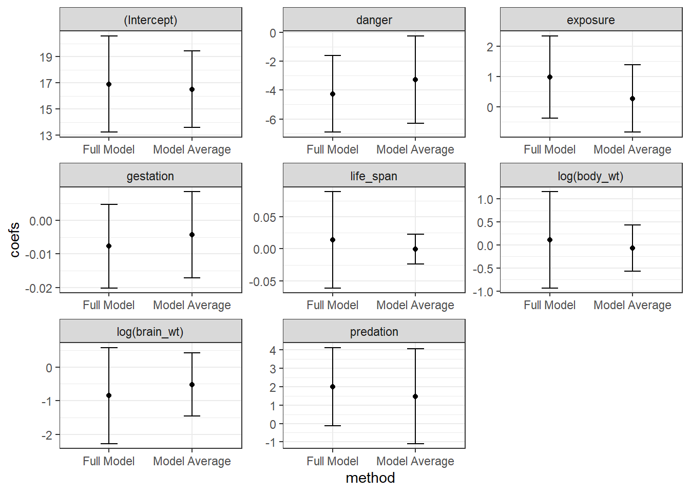
FIGURE 8.2: Comparison of full model and model-avaraged coefficient estimates and 95% confidence intervals
8.6 Regularization using penalization
As mentioned in the previous section, if your goal is prediction, it may be useful to shrink certain coefficients towards 0. One way to accomplish this goal is to add a penalty, \(\lambda \sum_{j=1}^p |\beta_j|^\gamma\), to the objective function used to estimate parameters (e.g., sum-of-squared errors or likelihood), where \(p\) is equal to the number of coefficients associated with our explanatory variables:
\[\sum_{i=1}^n(Y-\hat{Y}_i)^2 + \lambda \sum_{j=1}^p |\beta_j|^\gamma\]
Typically, \(\gamma\) is set to either 1 or 2, with \(\gamma=1\) corresponding to the “LASSO” (Least Absolute Shrinkage and Selection Operator) and \(\gamma=2\) corresponding to ridge regression. The two penalties can also be combined into what is referred to as the elastic net. When \(\lambda = 0\), we get the normal least-squares (or Maximum Likelihood) estimator34). As \(\lambda\) gets larger, coefficients will shrink towards 0. The degree of shrinkage will differ between the LASSO and Ridge regression estimators due to the difference in the penalty functions. When using the Lasso, some coefficients may actually equal 0 depending on the value of \(\lambda\), which allows some predictors to be dropped from the model. With Ridge regression, all coefficients will be retained. Thus, the two approaches perform very differently when faced with strong collinearity. The LASSO will usually select one of a set of collinear variables whereas Ridge regression will retain all variables but shrink their coefficients towards 0. Typically, a gridded set of \(\lambda\) values are considered and the value of \(\lambda\) that performs best (e.g., minimizes mean-squared prediction error is chosen).
Why do shrinkage estimators improve predictive performance? Essentially, shrinkage can be viewed as a method for reducing model complexity; shrinkage reduces variability in the estimates of \(\beta\) at the expense of introducing some bias (Hooten & Hobbs, 2015). This bias-variance tradeoff can be extremely effective in reducing prediction error, particularly when faced with too many predictors relative to the available sample size or in cases of extreme collinearity.
Below, we will estimate parameters using the LASSO and Ridge regression applied to the sleep data set. We will make use of the glmnet package (Friedman, Hastie, & Tibshirani, 2010), which works with matrices rather than dataframes. Therefore, we will first need to create our logged predictors of body and brain weight. We can specify \(\alpha = 1\) for the LASSO, \(\alpha = 0\) for Ridge regression and values in-between for the elastic net which combines both penalties.
library(glmnet)
mammalsc <- mammalsc %>% mutate(logbrain_wt = log(brain_wt),
                                logbody_wt = log(body_wt))
x = as.matrix(mammalsc[, c("life_span", "gestation", "logbrain_wt",
                           "logbody_wt", "predation", "exposure", "danger")])
fitlasso <- glmnet(x = x,
                   y= mammalsc$total_sleep, alpha=1)
By default, glmnet will estimate parameters across a range of \(\lambda\) values chosen in a smart way, but users can change the defaults. We can then inspect how the coefficient estimates (and number of coefficients in the model) change as we increase \(\lambda\) using the plot function with argument xvar = "lambda" (Figure 8.3).
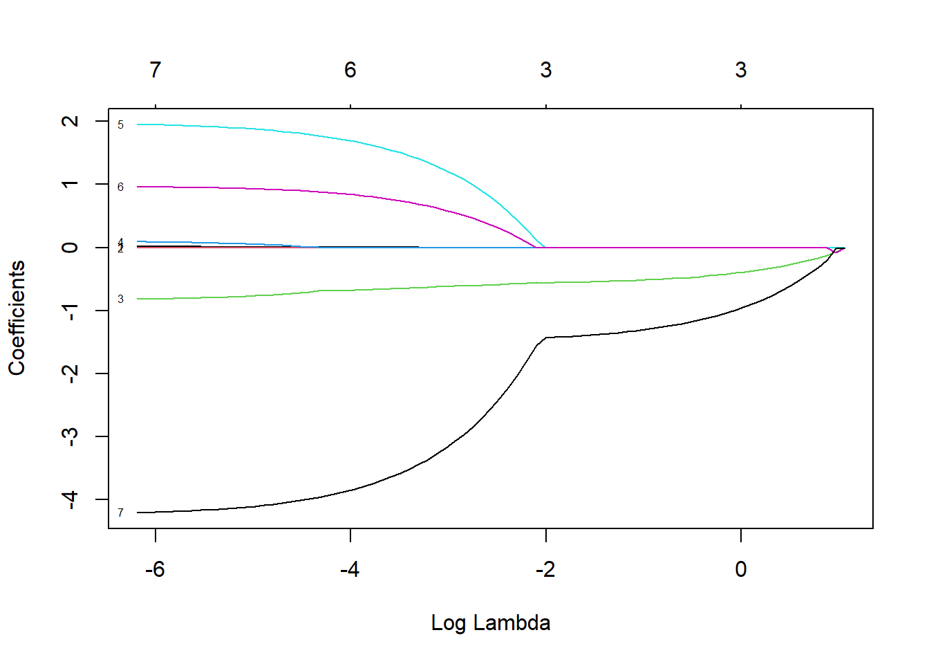
FIGURE 8.3: Coefficient estimates for predictors the sleep data set when using the LASSO with different values of \(\lambda\)
At this point, we have a number of different models, each with a different set of coefficient estimates determined by the unique set of \(\lambda\) values. We can see how the number of non-zero coefficients changes with \(\lambda\) and also the percent of the Deviance explained by the model (%Dev), which in the case of linear regression is equivalent to \(R^2\), using the print function.
##
## Call:  glmnet(x = x, y = mammalsc$total_sleep, alpha = 1)
##
##    Df  %Dev  Lambda
## 1   0  0.00 2.89600
## 2   4  8.32 2.63800
## 3   4 17.42 2.40400
## 4   3 24.79 2.19000
## 5   3 30.87 1.99600
## 6   3 35.92 1.81900
## 7   3 40.12 1.65700
## 8   3 43.60 1.51000
## 9   3 46.49 1.37600
## 10  3 48.89 1.25300
## 11  3 50.88 1.14200
## 12  3 52.54 1.04100
## 13  3 53.91 0.94820
## 14  3 55.05 0.86390
## 15  3 56.00 0.78720
## 16  3 56.78 0.71730
## 17  3 57.44 0.65350
## 18  3 57.98 0.59550
## 19  3 58.43 0.54260
## 20  3 58.80 0.49440
## 21  3 59.11 0.45050
## 22  3 59.37 0.41040
## 23  3 59.58 0.37400
## 24  3 59.76 0.34080
## 25  3 59.91 0.31050
## 26  3 60.03 0.28290
## 27  3 60.13 0.25780
## 28  3 60.21 0.23490
## 29  3 60.28 0.21400
## 30  3 60.34 0.19500
## 31  3 60.39 0.17770
## 32  3 60.43 0.16190
## 33  3 60.46 0.14750
## 34  3 60.49 0.13440
## 35  4 60.85 0.12250
## 36  5 61.60 0.11160
## 37  5 62.24 0.10170
## 38  5 62.76 0.09264
## 39  5 63.20 0.08441
## 40  5 63.57 0.07691
## 41  5 63.87 0.07008
## 42  5 64.12 0.06385
## 43  5 64.33 0.05818
## 44  5 64.51 0.05301
## 45  5 64.65 0.04830
## 46  5 64.77 0.04401
## 47  6 64.89 0.04010
## 48  6 64.99 0.03654
## 49  6 65.07 0.03329
## 50  6 65.13 0.03033
## 51  6 65.19 0.02764
## 52  6 65.24 0.02518
## 53  6 65.28 0.02295
## 54  6 65.31 0.02091
## 55  6 65.34 0.01905
## 56  6 65.36 0.01736
## 57  6 65.38 0.01582
## 58  6 65.39 0.01441
## 59  7 65.41 0.01313
## 60  7 65.43 0.01196
## 61  7 65.44 0.01090
## 62  7 65.45 0.00993
## 63  7 65.46 0.00905
## 64  7 65.47 0.00825
## 65  7 65.48 0.00751
## 66  7 65.48 0.00685
## 67  7 65.49 0.00624
## 68  7 65.49 0.00568
## 69  7 65.50 0.00518
## 70  7 65.50 0.00472
## 71  7 65.50 0.00430
## 72  7 65.50 0.00392
## 73  7 65.51 0.00357
## 74  7 65.51 0.00325
## 75  7 65.51 0.00296
## 76  7 65.51 0.00270
## 77  7 65.51 0.00246
## 78  7 65.51 0.00224
## 79  7 65.51 0.00204
Lastly, we can use cross-validation (see Section 8.7.1) to choose an optimal \(\lambda\). Cross-validation attempts to evaluate model performance by training the model on subsets of the data and then testing its predictions on the remaining data. This can be accomplished using the cv.glmnet function:
We can use the associated plot function to see how our estimates of mean-squared error change with \(\lambda\) (Figure 8.4):
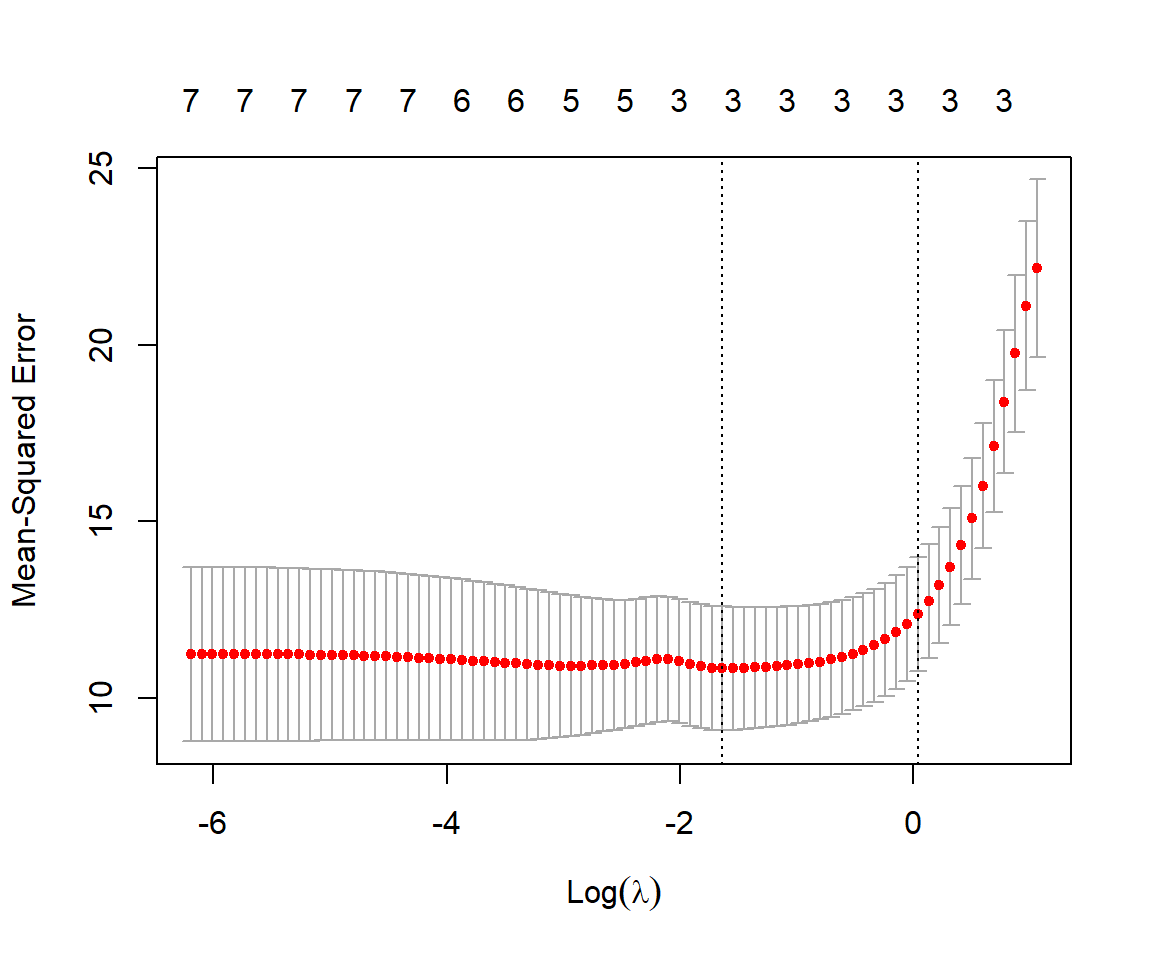
FIGURE 8.4: Mean-squared prediction error estimated using cross-validation with the sleep data set for different values of \(\lambda\).
For each value of \(\lambda\), the red dots and associated interval representing the estimated MSE along with \(\pm\) 1 SE. The left-most dotted line corresponds to the values of \(\lambda\) that minimizes the mean-squared error. The rightmost line gives the largest value of \(\lambda\) that results in an estimated MSE within 1SE of the minimum observed. Lastly, we can inspect the value of \(\lambda\) that gives the smallest MSE and also the resulting coefficients using:
## [1] 0.1949944## 8 x 1 sparse Matrix of class "dgCMatrix"
## s1
## (Intercept) 16.976166753
## life_span .
## gestation -0.008038413
## logbrain_wt -0.548365524
## logbody_wt .
## predation .
## exposure .
## danger -1.398245831We see that we are left with the same 3 predictors as the model with the lowest \(AIC_C\), but that their coefficients are also shrunk towards 0:
## Global model call: lm(formula = total_sleep ~ life_span + gestation + log(brain_wt) +
##     log(body_wt) + predation + exposure + danger, data = mammalsc)
## ---
## Model selection table
##    (Int)    dng log(brn_wt)   prd df   logLik  AICc delta weight
## 98  16.4 -3.628     -0.6763 1.992  5 -103.722 219.1     0      1
## Models ranked by AICc(x)
We can repeat the process using Ridge regression:
## [1] 1.408017## 8 x 1 sparse Matrix of class "dgCMatrix"
## s1
## (Intercept) 16.225126136
## life_span -0.008771936
## gestation -0.007109805
## logbrain_wt -0.314594126
## logbody_wt -0.181114581
## predation -0.193136879
## exposure -0.145969578
## danger -0.948772308In this case, all coefficients are non-zero. Lastly, we compare these coefficients to those from model-averaging and from the full model, below:
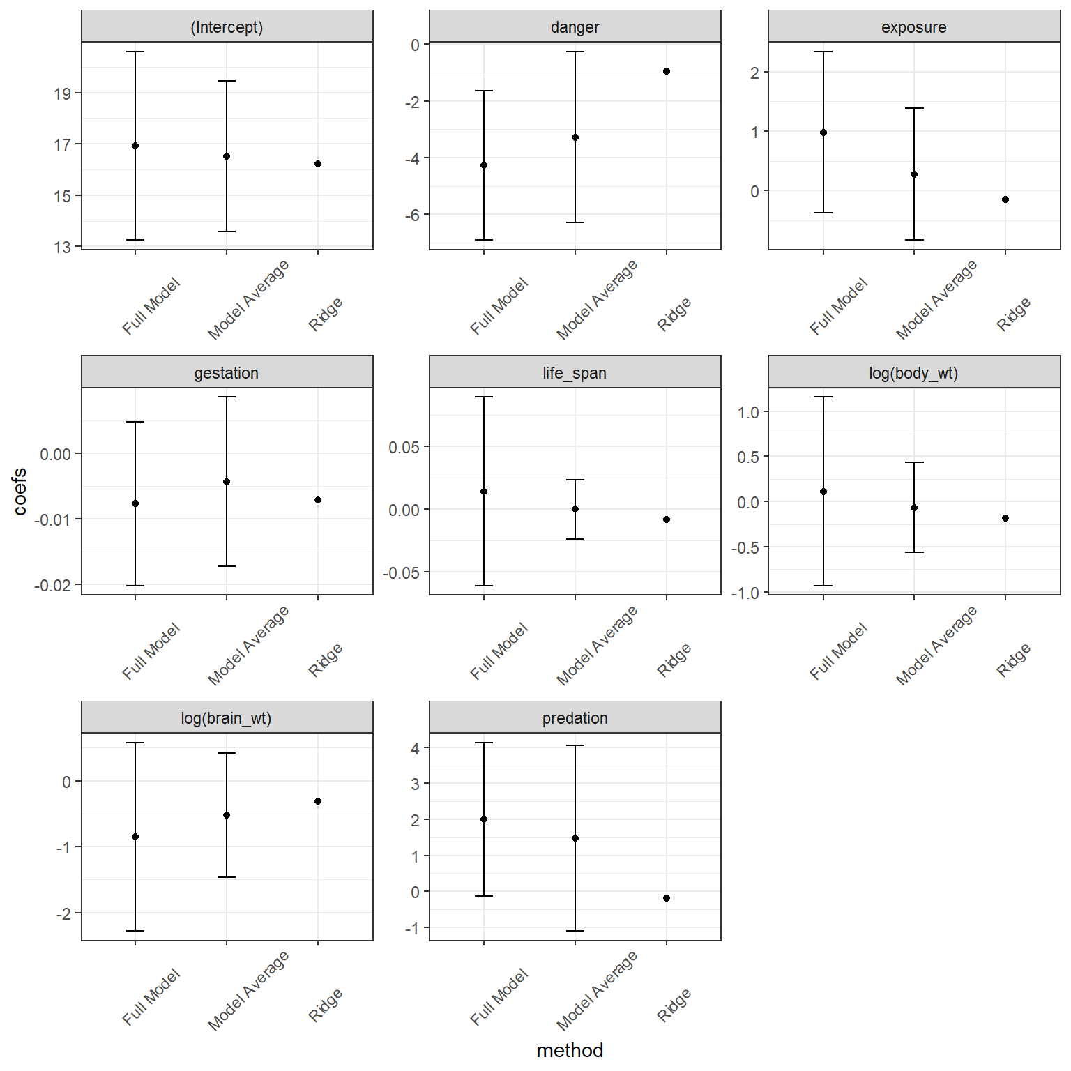
FIGURE 8.5: Comparison of full model, model-averaged and LASSO coefficients.
We again see that the coefficients from Ridge regression are shrunk towards 0, in this case more so than model averaging. One challenge with penalization-based methods is that it is not straightforward to calculate appropriate confidence intervals due to the bias introduced by the penalization, and therefore glmnet does not supply SEs. In many ways, a Bayesian treatment of regularization seems more natural in that the penalization terms can be viewed as arising from specific prior specifications (Casella, Ghosh, Gill, & Kyung, 2010; Tibshirani, 2011). For a fuller treatment of regularization methods and connections between the Lasso, Ridge Regression, and Bayesian methods, see Hooten & Hobbs (2015).
8.7 Evaluating model performance
We have now seen a few different modeling strategies, identified some of the challenges inherent to them, including the potential of overfitting data, and discussed ways that we can improve predictive performance via shrinkage of coefficients towards 0. It is also important that we have tools for evaluating models and modeling strategies. Two powerful approaches are cross-validation, which was briefly mentioned in the previous section, and bootstrapping.
8.7.1 Cross-validation
One potential issue with evaluating models via data splitting (i.e., the approach I used during my Linear Regression mid-term; Section 8.2) is that estimates of model performance can be highly variable depending on how observations get partitioned into training and test data sets. One way to improve upon this approach is to use \(k\)-fold cross validation in which the data are partitioned into \(k\) different subsets, referred to as folds (Mosteller & Tukey, 1968). The model is then trained using all data except for 1 of the folds which serves as the test data set. This process is then repeated with each fold used as the test data set. The steps are as follows:
- Split the data into many subsets (\(D_i = 1, 2, \ldots k\)).
- Loop over \(i\):
- Fit the model using data from all subsets except \(i\). We will use a \(_{-i}\) subscript to refer to subsets that include all data except those in the \(i^{th}\) fold (e.g., \(D_{-i}\)).
- Predict the response for data in the \(i^{th}\) fold: \(\hat{Y}_{i}\).
- Pool results and evaluate model performance, e.g., by comparing \(Y_i\) to \(\hat{Y}_i\) (\(i = 1, 2, \ldots, n\)).
We will demonstrate this process using functions in the caret package (Kuhn, 2021), though it is also easy to implement the approach on your own (e.g., using a for loop). The caret package allows one to implement various forms of data partitioning/resampling via its trainControl function. Here, we will specify that we want to evaluate the performance using cross-validation (method = "cv") with 10 folds (number = 10). Let’s evaluate the model containing our same set of sleep predictors.
library(caret)
set.seed(1045) # to ensure we get the same result every time.
# defining training control
# as cross-validation and
# value of K equal to 10
train_control <- trainControl(method = "cv",
                              number = 10)

# training the model by assigning sales column
# as target variable and rest other column
# as independent variable
model <- train(total_sleep ~ life_span + gestation + log(brain_wt) +
                 log(body_wt) + predation + exposure + danger,
               data = mammalsc,
               method = "lm",
               trControl = train_control)

# printing model performance metrics
# along with other details
print(model)
## Linear Regression
##
## 42 samples
## 7 predictor
##
## No pre-processing
## Resampling: Cross-Validated (10 fold)
## Summary of sample sizes: 36, 38, 38, 38, 38, 38, ...
## Resampling results:
##
## RMSE Rsquared MAE
## 3.598593 0.5286154 3.001091
##
## Tuning parameter 'intercept' was held constant at a value of TRUEWe can repeat this approach multiple times (referred to as repeated k-fold cross validation) by changing the method argument of trainControl to repeatedcv and by specifying how many times we want to repeat the process using the repeats argument.
train_control <- trainControl(method = "repeatedcv",
                              number = 10, repeats=5)

# training the model by assigning sales column
# as target variable and rest other column
# as independent variable
model <- train(total_sleep ~ life_span + gestation + log(brain_wt) +
                 log(body_wt) + predation + exposure + danger,
               data = mammalsc,
               method = "lm",
               trControl = train_control)

# printing model performance metrics
# along with other details
print(model)
## Linear Regression
##
## 42 samples
## 7 predictor
##
## No pre-processing
## Resampling: Cross-Validated (10 fold, repeated 5 times)
## Summary of sample sizes: 37, 38, 38, 39, 38, 36, ...
## Resampling results:
##
## RMSE Rsquared MAE
## 3.328851 0.6342511 2.792544
##
## Tuning parameter 'intercept' was held constant at a value of TRUEWe can compare these results to the estimate \(R^2\) and RMSE (equivalent to \(\hat{\sigma}\) when using linear regression) from the fit of our full model.
## [1] 0.6551552## [1] 3.036907We see that the cross-validation estimate of \(R^2\) is smaller and the estimate of \(\hat{\sigma}\) is larger than the estimates provided by lm. Although the differences are small here, cross-validation can be particularly useful for estimating out-of-sample performance (i.e., performance of the model when applied to new data not used to fit the model) when model assumptions do not hold. For example, most ecological data sets are subjected to some form of correlation due to repeated observations on the same sample unit or spatial or temporal autocorrelation, and thus, observations will not be independent. When applying cross-validation to data with various forms of dependencies, it is important to create folds that are independent of each other (Roberts et al., 2017); the data within folds, however, can be non-independent. For spatial or temporal data, this can often be accomplished by creating blocks of data that clustered in space or time. Several R packages have been developed to facilitate spatial cross-validation, including sperrorest (Brenning, 2012), ENMeval (Kass et al., 2021), and blockCV (Valavi, Elith, Lahoz-Monfort, & Guillera-Arroita, 2019).
8.7.2 Boostrapping to evaluate model stability
So far, we have looked at how we can evaluate model performance using cross-validation. This process attempts to evaluate model performance when applied to a new data set. Our examples in the last section assumed we had a pre-specified model. What if we wanted to also evaluate the impact of various modeling choices along the way – e.g., stepwise selection procedures or tuning parameters (e.g., \(\lambda\)) used in regularization methods? We could repeat these steps (model selection, model tuning) with each fold. Similarly, we could evaluate model performance and also modeling strategies using bootstrap resampling. In this section, we will highlight a bootstrap approach implemented in the rms package (Harrell Jr, 2021).
To evaluate model performance using a bootstrap, we will use mimic the entire process from start to finish, including:
- creating training and test data sets using separate bootstraps.
- train the model using the training data (this step could include choosing tuning parameters or using stepwise selection algorithms to determine a final model).
- evaluate the model using the test data
To estimate model performance metrics (Figure 8.6A), we begin by estimating the average degree of optimism resulting from evaluating the model using the same data as was used to train the model. We then subtract this optimism from the same performance metrics calculated using the full data set.
- Fit a model to the full data set and estimate \(R^2\).
- Form bootstrapped test and bootstrapped training data sets by resampling the original data set with replacement
- Fit the full model to the bootstrapped training data set and estimate \(R^2_{trian}\).
- Use the model from step 3 to form predictions for the test data set.
- Use the predictions from step 4 and the test data to estimate \(R^2_{test}\).
- Estimate the degree of optimism, \(\delta_i = R^2_{train}- R^2_{test}\).
- Estimate an improved \(R^2\) by subtracting the average optimism across the different bootstrap replicates from the \(R^2\) in step 1.
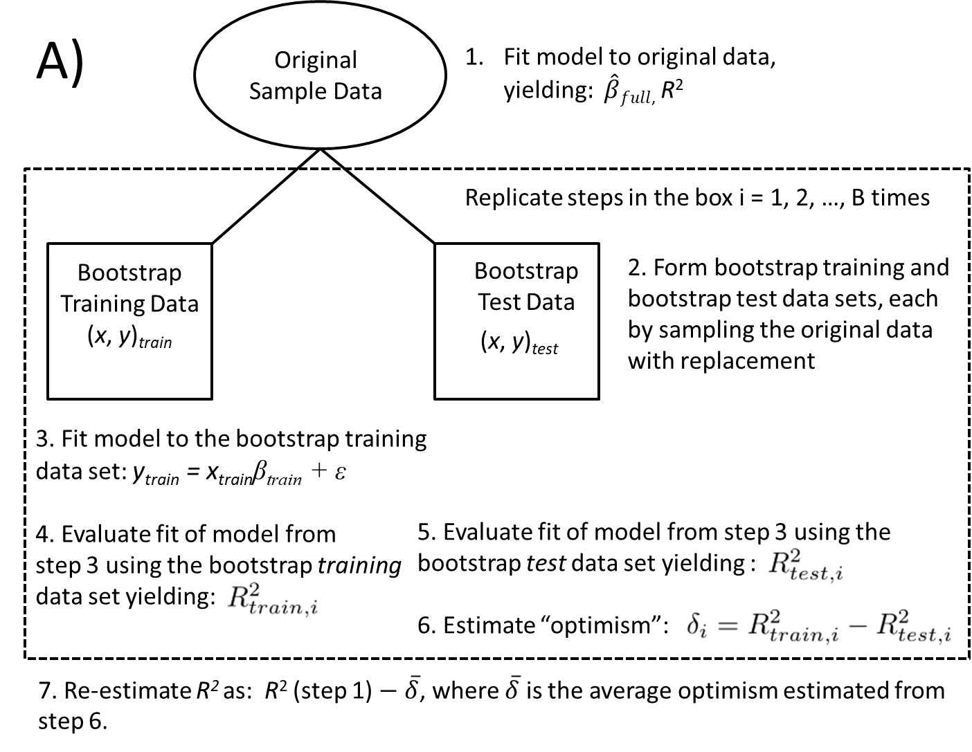

We can also use a bootstrap to recalibrate our predictions. If we have overfit the data, it may help to shrink our predictions back towards the mean response in the data set (Figure 8.6B). We can estimate the degree of shrinkage by comparing how well our predictions from models fit to the training data match observations in the test data set:
- Estimate regression parameters using the full data set.
- Form bootstrapped test and bootstrapped training data sets by resampling the original data set with replacement
- Fit the full model to the bootstrapped training data set
- Use the model from step 3 to form predicted responses for the bootstrapped test data set.
- Fit a linear regression model using the test data responses (as the response variable) and the predicted values from step 4 as the only explanatory variable
- Repeat steps 2-5 many times. The average slope in step 5 can be used to proportionally reduce, or shrink, the regression parameters from step 1 towards 0; if no overfitting has occurred, the average slope in step 5 will be 1.
The rms package has functions for evaluating a variety of models (see below), including those obtained by backwards selection. However, users must fit their models using functions specific to the rms package:
- linear regression models (using
olsrather thanlm) - generalized least squares (using
Glsrather thangls) - logistic regression models (using
lrmrather thanglm) - cox proportional hazards models (using
cpmrather thancph)
Unfortunately, it does not implement methods for mixed effect models, which we will encounter later (see Section [add reference]).
Let’s explore this approach with the sleep data. We must first fit the model using ols. We can then evaluate model performance when also including backwards selection using the validate function with the argument bw = TRUE.
library(rms)
set.seed(130)
fullmod.ols<-ols(total_sleep ~ life_span + gestation + log(brain_wt) +
                   log(body_wt) + predation + exposure + danger,
               data = mammalsc, x = TRUE, y = TRUE)
  validate(fullmod.ols, bw = TRUE)
##
## Backwards Step-down - Original Model
##
## Deleted Chi-Sq d.f. P Residual d.f. P AIC R2
## body_wt 0.04 1 0.8326 0.04 1 0.8326 -1.96 0.655
## life_span 0.11 1 0.7448 0.15 2 0.9275 -3.85 0.654
## gestation 1.32 1 0.2500 1.47 3 0.6883 -4.53 0.640
## exposure 1.76 1 0.1845 3.23 4 0.5193 -4.77 0.622
## predation 3.66 1 0.0557 6.90 5 0.2284 -3.10 0.585
##
## Approximate Estimates after Deleting Factors
##
## Coef S.E. Wald Z P
## Intercept 17.4416 1.0680 16.331 0.000e+00
## brain_wt -0.9194 0.1974 -4.658 3.199e-06
## danger -1.5755 0.3566 -4.418 9.977e-06
##
## Factors in Final Model
##
## [1] brain_wt danger## index.orig training test optimism index.corrected n
## R-square 0.5852 0.6279 0.5205 0.1074 0.4778 40
## MSE 8.9805 7.2317 10.3815 -3.1498 12.1303 40
## g 4.1115 4.0430 3.9206 0.1223 3.9892 40
## Intercept 0.0000 0.0000 0.6651 -0.6651 0.6651 40
## Slope 1.0000 1.0000 0.9432 0.0568 0.9432 40
##
## Factors Retained in Backwards Elimination
##
## life_span gestation brain_wt body_wt predation exposure danger
## * * * *
## * *
## * * *
## * *
## * *
## * * * * *
## *
## * *
## * * *
## * * *
## * *
## * *
## * *
## * * * *
## * *
## * *
## * *
## * * *
## * *
## * *
## * *
## * * *
## *
## * * *
## * *
## * *
## * * *
## * *
## * *
## * *
## * *
## * * * *
## * * *
## * * *
## * * *
## * *
## * *
## * *
## * *
## * * * * *
##
## Frequencies of Numbers of Factors Retained
##
## 1 2 3 4 5
## 2 23 10 3 2We see that backwards elimination results in a fair degree of optimism. Correcting for it decreases our estimate of \(R^2\) and increases our estimate of the Mean-Squared Error. The estimates of intercept and slope also tell us that we can improve prediction error by recalibrating our model, shrinking our original estimates, \(\hat{Y}_i^{naive}\), towards the overall mean using \(\hat{Y}^C_i = 0.6651 + 0.9432\hat{Y}_i^{naive}\). The validate function also shows us which predictors are chosen when the backwards selection algorithm is applied to each bootstrap sample. We see that there is quite a bit of variability in the final model that is chosen. Thus, if we were to collect another data set of the same size and apply the same model-selection algorithm, we might vary well end up with a different set of variables in the reduced model. We may choose to communicate this uncertainty due to model selection by reporting bootstrap inclusion frequencies (how often variables are selected in final models) or by listing other “competitive models” (i.e, those models that are frequently chosen) (Heinze et al., 2018).
8.8 Summary
In this section, we have presented several modeling strategies, including:
- Stepwise selection algorithms (possibly with change-in-estimate criterion)
- Full model inference (df spending)
- Model averaging (using multiple models for inference)
- Penalized estimation methods (LASSO, Ridge regression)
For describing associations, we may consider any of these methods including the use of a full model or stepwise-selection algorithms. Note, however, that interpretation of coefficients can be more challenging when using model-averaging or regularization/penalization due to the bias introduced when estimating regression coefficients with shrinkage. These latter methods are geared towards improving predictions. For inference, we are likely best off fitting a small number of informed models (e.g., representing different causal mechanisms) which we can then compare. Lastly, we have seen how cross-validation and bootstrap resampling methods can help us quantify how (possibly tuned) models will likely perform when applied to new data. There is tremendous demand for analysts that can develop good predictive models, and this has fueled the development of open-source software for tuning and evaluating models. In addition to the tools available in the caret package (Kuhn, 2021), the tidymodels and workflows packages offer powerful options for evaluating models using resampling-based techniques (Kuhn & Wickham, 2020; Vaughan, 2021). Useful tutorials for these packages can be found here and here.
Albumin is sometimes used as an indicator of kidney disease.↩
The overall type I error is the probability of rejecting one or more null hypotheses when all of them are true↩
If all of our assumptions of linear regression hold, then least squares will give us the Maximum Likelihood estimate - see later section↩