Chapter 20 Generalized Estimating Equations (GEE)
Learning Objectives
- Learn how to model population-level response patterns for count and binary data using Generalized Estimating Equations (GEEs)
20.1 Introduction to Generalized Estimating Equations
In the last section, we saw how the parameters in typical GLMMs have a subject-specific interpretation. We also saw how we could estimate mean-response patterns at the population level by integrating over the distribution of the random effects. Lastly, we saw how we could use the marginal_coef function in the GLMMadaptive package to estimate parameters describing marginal (i.e., population-average) mean-response patterns from fitted GLMMS.
There are times, however, when we may be interested in directly modeling how the population mean changes as a function of our predictor variables. For Normally distributed response variables, we can use the gls function in the nlme package, which allows us to specify various correlation structures for our residuals (Section 19.2.2). Yet, as we highlighted in Section 19.3, multivariate distributions for count and binary data do not have separate mean and variance parameters, making it challenging to fit marginal models to binary or count data in the case where we have repeated measures. Simply put, there is no multivariate Poisson or Binomial distribution that contains separate parameters for describing correlation among observations from the same cluster, so we cannot take a simple marginal modeling approach as we saw for Normally distributed data (see Sections 18.13 and 19.2.2).
Generalized Estimating Equations (GEEs) offer an alternative approach to modeling correlated binary or count data in which one specifies a model for the first two moments (the mean and variance) of the data but not the full marginal distribution (Zeger et al., 1988; Hilbe & Hardin, 2008; Fieberg et al., 2009). Parameters are estimated by solving:
\[\begin{equation} \sum_{i=1}^n \frac{\partial \mu_i}{\partial \beta}V_i^{-1}(Y_i - \mu_i) = 0, \text{where} \tag{20.1} \end{equation}\]
\(Y_i = (Y_{i1}, Y_{i2}, \ldots, Y_{im_i})\) denotes the vector of response data for individual \(i\), \(\mu_i = g^{-1}(X_i\beta)\) represents the mean response as a function of covariates and regression parameters, and \(\frac{\partial \mu_i}{\partial \beta}\) is an \(m_i \times p\) matrix of first derivatives of \(\mu_i\) with respect to \(\beta\). The variance-covariance matrix for subject \(i\), \(V_i\), is typically modeled by adopting a common form for the variance based on an appropriate member of the exponential family, combined with a “working correlation model” to describe within-subject dependencies. We can write \(V_i = A_i^{1/2}R_i(\alpha)A_i^{1/2}\) where \(A_i\) captures the assumed standard deviations, and \(R_i\) is our working correlation model that describes within subject correlation and may include additional parameters, \(\alpha\). It is common to assume \(A_i = \sqrt{\mu_i(1-\mu_i)}\) for binary data and \(A_i = \sqrt{\mu_i}\) for count data. Typical examples of working correlation assumptions include independence, compound symmetry (see Section 18.13), or a simple (ar1) auto-regressive model for temporal data.
Importantly, estimates of the regression parameters will be (asymptotically) unbiased even when the working correlation and variance model is mis-specified, provided that the model for the marginal mean is correct and the mechanisms responsible for any missing data or sample-size imbalance can be assumed to be completely random (Zeger et al., 1988); proper specification of \(V_i\) should increase precision. Separate analyses using multiple working correlation matrices could be used as a sort of sensitivity analysis, or one can use various tools (e.g., lorelograms; Heagerty & Zeger, 1998; Iannarilli et al., 2019) to determine an appropriate correlation structure. The sampling distribution of the regression parameter estimators will approach that of a normal distribution as the number of clusters (\(i\)) goes to infinity. Robust(“sandwich”) standard errors that assume clusters are independent are typically used when forming confidence intervals or conducting hypothesis tests (White, 1982; Liang & Zeger, 1986).
20.2 Motivating GEEs
You may be wondering where equation (20.1) comes from. In Section 10.10 we saw that the maximum likelihood estimator for the linear model is equivalent to the least-squares estimator, which finds the values of \(\beta\) that minimize:
\[\begin{gather} \sum_{i=1}^n \frac{(Y_i - (\beta_0+X_{1i}\beta_1+\ldots))^2}{2\sigma^2} = \sum_{i=1}^n \frac{(Y_i - \mu_i)^2}{2\sigma^2} \end{gather}\]
Taking the derivative with respect to \(\beta\) and setting the result to 0, gives:
\[\begin{gather} \sum_{i=1}^n \frac{(Y_i -\mu_i)}{\sigma^2} \frac{\partial \mu_i}{\partial \beta} = 0, \text{ or equivalently,} \sum_{i=1}^n \frac{\partial \mu_i}{\partial \beta}V_i^{-1}(Y_i -\mu_i) = 0, \end{gather}\]
where \(V_i = Var[Y_i |X_i]= \sigma^2\). Similarly, for generalized linear models (e.g., logistic and Poisson regression), it turns out that maximum likelihood estimators are found by solving:
\[\begin{equation} \sum_{i=1}^n \frac{\partial \mu_i}{\partial \beta}V_i^{-1}(Y_i - \mu_i) = 0 \tag{20.2} \end{equation}\]
To demonstrate this fact, we will derive this result for the logistic regression model, which assumes:
\[\begin{gather} Y_i \sim Bernoulli(\mu_i) \\ \mu_i = g^{-1}(X_i\beta) = \frac{e^{x_i\beta}}{1+e^{x_i\beta}} \end{gather}\]
First, note that for the logistic regression model:
\[\begin{gather} \frac{\partial \mu_i}{\partial \beta} = \frac{X_i e^{X_i\beta}\left(1+e^{X_i\beta}\right)- X_ie^{X_i\beta}e^{X_i\beta}}{\left(1+e^{X_i\beta}\right)^2} \\ = \frac{X_i e^{X_i\beta}}{\left(1+e^{X_i\beta}\right)^2} \end{gather}\]
Furthermore:
\[\begin{gather} V_i = \mu_i (1-\mu_i) = \left(\frac{e^{X_i\beta}}{1+e^{X_i\beta}}\right)\left(1-\frac{e^{X_i\beta}}{1+e^{X_i\beta}}\right)\\ = \left(\frac{e^{X_i\beta}}{1+e^{X_i\beta}}\right)\left(\frac{1}{1+e^{X_i\beta}}\right) \\ = \frac{e^{X_i\beta}}{\left(1+e^{X_i\beta}\right)^2} \end{gather}\]
Thus, \(\frac{\partial \mu_i}{\partial \beta}V_i = X_i\) and equation (20.2) can be simplified to:
\[\begin{gather} \sum_{i=1}^n X_i \left(Y_i - \frac{e^{X_i\beta}}{1+e^{X_i\beta}}\right) = 0 \tag{20.3} \end{gather}\]
We can show that we end up in the same place if we take the derivative of the log-likelihood with respect to \(\beta\) and set the expression to 0. The likelihood of the data is thus given by:
\[\begin{gather} L(\beta; Y) = \prod_{i=1}^n \mu_i^{Y_i}(1-\mu_i)^{1-Y_i} \\ = \prod_{i=1}^n \left(\frac{e^{X_i\beta}}{1+e^{x_i\beta}}\right)^{Y_i}\left(1-\frac{e^{X_i\beta}}{1+e^{X_i\beta}}\right)^{1-Y_i}\\ = \prod_{i=1}^n \left(\frac{e^{X_i\beta}}{1+e^{X_i\beta}}\right)^ {Y_i}\left(\frac{1}{1+e^{X_i\beta}}\right)^{1-Y_i} \\ = \prod_{i=1}^n \left(e^{x_i\beta}\right)^{Y_i}\left(\frac{1}{1+e^{X_i\beta}}\right) \end{gather}\]
Thus, the log-likelihood is given by:
\[\begin{gather} log L(\beta; Y) = \sum_{i=1}^n Y_i(X_i\beta) - \sum_{i=1}^n \log \left(1+e^{X_i\beta}\right) \tag{20.4} \end{gather}\]
Taking the derivative of the log-likelihood with respect to \(\beta\) and setting the expression equal to 0 gives us:
\[\begin{gather} \frac{\partial log L(\beta; Y)}{\partial \beta} = \sum_{i=1}^n X_iY_i - \sum_{i=1}^n \frac{1}{1+e^{X_i\beta}}e^{X_i\beta}X_i =0 \\ = \sum_{i=1}^n X_i\left(Y_i - \frac{e^{X_i\beta}}{1+e^{X_i\beta}}\right) =0, \end{gather}\]
which is the same as equation (20.3).
If you found this exercise to be fun, you might follow up by proving that the maximum likelihood estimator for Poisson regression is also equivalent to equation (20.2).
What is the point of all this? The equations used to estimate parameters in linear models and generalized linear models take a similar form. Generalized estimating equations (eq. (20.1)) extend this basic idea to situations where we have multiple observations from the same cluster. We just replace \(V_i\) with a variance covariance matrix associated with the observations from the same cluster.
20.3 GEE applied to our previous simulation examples
There are a few different packages for fitting GEEs in R. We will explore the geeglm function in the geepack package (Yan, 2002; Halekoh, Højsgaard, & Yan, 2006). Let’s revisit our hockey skaters from Section (glmm). Let’s assume the observations from the same skater are all exchangeable, giving a compound symmetry correlation structure:
\[\begin{equation} R(\alpha) = \begin{bmatrix} 1 & \alpha & \cdots & \alpha \\ \alpha & \ddots & \ddots & \vdots \\ \vdots & \ddots & \ddots & \alpha \\ \alpha & \cdots & \alpha & 1 \end{bmatrix} \tag{20.5} \end{equation}\]
Further, as with logistic regression, we will assume:
- \(E[Y_i | X_i ] = \frac{e^{X_i\beta}}{1+e^{X_i\beta}}\)
- \(Var[Y_i|X_i] = E[Y_i | X_i ](1-E[Y_i | X_i ])\)
We specify this assumption using the family = binomial() argument. Note, however, that we are not assuming our data come from a binomial distribution. We only adopt the mean and variance assumptions from logistic regression. Further, note that our model differs from those of the corresponding GLMMs with a random intercept (from Section 19) in that we are modeling the population mean as a logit-linear In addition, we have to specify our clustering variable, individual using id = individual.
fit.gee.e <- geeglm(Y ~ practice.num, family = binomial(),
                    id = individual, corstr = "exchangeable",
                    data = skatedat)
summary(fit.gee.e)
##
## Call:
## geeglm(formula = Y ~ practice.num, family = binomial(), data = skatedat,
## id = individual, corstr = "exchangeable")
##
## Coefficients:
## Estimate Std.err Wald Pr(>|W|)
## (Intercept) -3.4833 0.2708 165.4 <2e-16 ***
## practice.num 0.5960 0.0421 200.4 <2e-16 ***
## ---
## Signif. codes: 0 '***' 0.001 '**' 0.01 '*' 0.05 '.' 0.1 ' ' 1
##
## Correlation structure = exchangeable
## Estimated Scale Parameters:
##
## Estimate Std.err
## (Intercept) 0.979 0.1663
## Link = identity
##
## Estimated Correlation Parameters:
## Estimate Std.err
## alpha 0.2619 0.06906
## Number of clusters: 100 Maximum cluster size: 10If we compare the coefficients from the GLMM with a random intercept to the coefficients from the Generalized Estimating Equations approach, we find that the latter are closer to 0.
##  (Intercept) practice.num
##       -5.949        0.997
This result was to be expected since the GLMM estimates subject-specific parameters whereas we are directly modeling the population-averaged response pattern using GEEs. Thus, we see that unlike the GLMM, the GEE does a nice job of estimating the proportion of skaters in the population that can skate backwards at each practice (Figure
mdat6<-rbind(mdat5,
             data.frame(practice.num = practice.num,
                        p = plogis(marginal_beta$betas[1]+practice.num * marginal_beta$betas[2]),
                        type = rep("GEE", 10)))

# Plot
ggplot(mdat6, aes(practice.num, p, col=type)) +
  geom_line() + geom_point() +
  xlab("Number of practices") +
  ylab("Proportion of skaters that can skate backwards")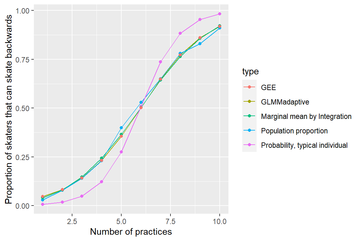
FIGURE 20.1: (ref geefigureref)
Similarly, a GEE with an exchangeable working correlation structure does a nice job estimating the population-mean-response pattern for our simulated birders (Figure 20.2:
geebird <- geeglm(Y ~ lobs.time, family = poisson(),
                  id = individual, corstr = "exchangeable", data = birdobs)

# Summarize the mean number of birds seen as a function of lobs.time at the population-level
mdatb$gee <- exp(coef(geebird)[1] + mdatb$lobs.time*coef(geebird)[2])

# plot
ggplot(mdatb, aes(lobs.time, meanY)) + geom_point() +
  geom_line(aes(lobs.time, gee), color="black") +
  xlab("log(Observation time)") + ylab("Number of birds seen")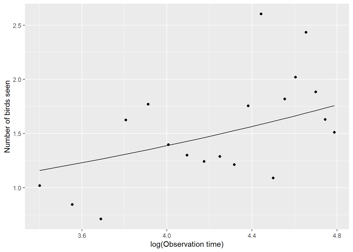
FIGURE 20.2: Population mean response curve describing the number of birds seen as a function of log observation time in the population of students. Mean response curve was estimated using a Generalized Estimating Equation with exchageable working correlation. Points are the empirical means at each observation level.
20.4 GEEs versus GLMMs
Given that GLMMs and GEEs estimate parameters that have different interpretations, much of the literature that aims to provide guidance on choosing between these methods focuses on the estimation target of interest - i.e., whether one is interested in describing subject-specific response patterns (GLMM) or population-average response patterns (GEE). Yet, we saw that it is possible to estimate population-average response patterns from GLMMs if we integrate over the distribution of the random effects, so the choice of estimation target may not be a deciding factor when choosing between GEEs and GLMMs. In this short section, we further contrast the two approaches in hopes of providing additional guidance to practitioners.
Complexity: GLMMS require approximating an integral in the likelihood before parameters can be estimated (Section 19.6). This makes GLMMs much more challenging to fit than GEEs. On the other hand, GLMMs can describe much more complex hierarchical data structures (e.g., clustering due to multiple grouping variables - such as individual and year), whereas GEEs typically only allow for a single clustering variable.
Robustness: GLMMs require distributional assumptions (e.g., Normally distributed random effects, a distribution for \(Y\) conditional on the random effects). GEEs, by contrast, only make assumptions about the mean and variance/covariance of the data, and estimates should be robust to incorrect assumptions about the variance/covariance structure. On the other hand, GEEs have more strict requirements when it comes to missing data. Whereas standard applications of GEE require data to be missing completely at random, likelihood approaches are still appropriate if missingness depends only on the individual’s observed data (i.e. their covariates and their other response values) and not on data that were not observed (e.g. the missing response) (Carrière & Bouyer, 2002; Little & Rubin, 2019).
Tools for model selection and inference: since GLMMs are likelihood based, we have a number of methods that can be used to compare and select an appropriate model (e.g., AIC, likelihood ratio tests). We can also assess goodness-of-fit using simulation-based methods. Further, we can simulate future responses and estimate prediction intervals. Since GEEs only make assumptions about the mean and variance of the data, we cannot use likelihood-based methods for comparing models.