A Projects and Reproducible Reports in R
Much of this section was lifted from Rafeal A. Irizarry’s Introduction to Data Science: Data Analysis and Prediction Algorithms with R, which can be found here: https://rafalab.github.io/dsbook/
The material in his book (and thus, this chapter) is licensed under the Creative Commons Attribution-NonCommercial-ShareAlike 4.0 International CC BY-NC-SA 4.0.
I have added a few initial sections related to R and Rstudio. In addition, I made a few minor changes in places to simplify the text, provide connections to the rest of the book, and to also fill in spots where I thought additional information would be useful.
A.1 Introduction to R and RStudio
We will use R and Rstudio throughout to learn the statistical concepts discussed in the textbook. Many new users are often confused about the difference between R and Rstudio (many students list Rstudio on their CV, when it is probably more important to list R or both R and Rstudio!). R is the name of the programming language itself and RStudio is a graphical user interface (or GUI) used to interact with R. Rstudio lets us run R in an enhanced working environment by providing us with additional functionality (e.g., menu options, multiple windows for plots, code, help files, etc.).
The panel in the upper right contains your workspace as well as a history of the commands that you’ve previously entered. Any plots that you generate will show up in the panel in the lower right corner.
The panel on the left is where the action happens. It’s called the console. Every time you launch RStudio, it will have the same text at the top of the console telling you the version of R that you’re running. Below that information is the prompt. As its name suggests, this prompt is really a request, a request for a command. Initially, interacting with R is all about typing commands and interpreting the output.
You can name and store results in objects using either an equal sign (=) or an arrow (<-); we will use the latter throughout this book. For example, we can store a vector containing the numbers 1, 2, and 3 (generated by typing 1:3 in R) into an object called a using:
To refer to the stored object, we can just Type its name (a in this case):
## [1] 1 2 3This will display the object we created. We can also use a in future calculations. For example, we can add 2 to all of these numbers by typing:
## [1] 3 4 5For more complex problems, you will want to write code in a file that we can save, share, and access at a later point in time.
A.1.1 Installing packages and accessing data
Many users contribute code to do all sorts of things in R. They do this by writing `packages’ (bundles of code, sometimes combined with data) and making them available for public download. Accessing this code requires 2 steps:
A. The package has to be downloaded (“installed”) onto your computer. This step can be accomplished using the function install.packages() or via the menus in RStudio (Tools -> Install Packages). Packages only need to be installed once.
B. Each time we open R, we have to “tell R” if we want to use any of the add-on packages that we have downloaded. We do this by typing library(packagename) (replacing packagename with the name of the package we are interested in using).
Note that we can also access specific functions in packages by using package-name::function-name. For example, dplyr::summarize will use the the summarize function in the dplyr package (Wickham et al., 2021). This syntax will be useful when we want to highlight which package contains the function we are using. It can also be critical in cases where we have loaded more than 1 package that contains a function with the same name (e.g., there is also a summarize function in the plyr package).
A.2 Reproducible projects with RStudio and R markdown
The final product of any data analysis project is often a report or scientific publication containing a description of the findings along with some figures and tables resulting from the analysis. Imagine that after you finish your analysis and the report, you are told that you were given the wrong data set. You thus need to run the same analysis with a new data set. Similarly, you may realize that a mistake was made and need to re-examine the code, fix the error, and re-run the analysis. Or, perhaps your advisor or a researcher from another group studying the same phenomenon would like to see your code and be able to reproduce the results to learn about your approach.
Situations like the ones just described are actually quite common for a data scientist. Here, we describe how you can keep your data science projects organized with RStudio so that re-running an analysis is straight-forward. We then demonstrate how to generate reproducible reports with R markdown and the knitR package in a way that will greatly help with recreating reports with minimal work. This is possible due to the fact that R markdown documents permit code and textual descriptions to be combined into the same document, and the figures and tables produced by the code are automatically added to the document.
A.3 RStudio projects
RStudio provides a way to keep all the components of a data analysis project organized. In this section we quickly demonstrate how to start a new a project and some recommendations on how to keep these organized. RStudio projects also permit you to have several RStudio sessions open and keep track of which is which.
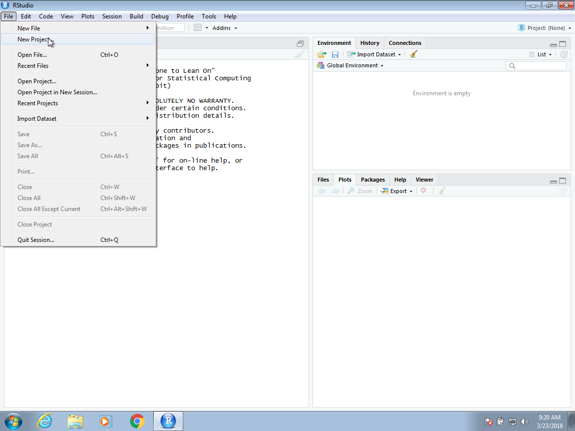
To start a project, click on File and then New Project. Often, we have already created a folder to save the work. If so, we select Existing Directory. Here we show an example in which we have not yet created a folder and select the New Directory option.
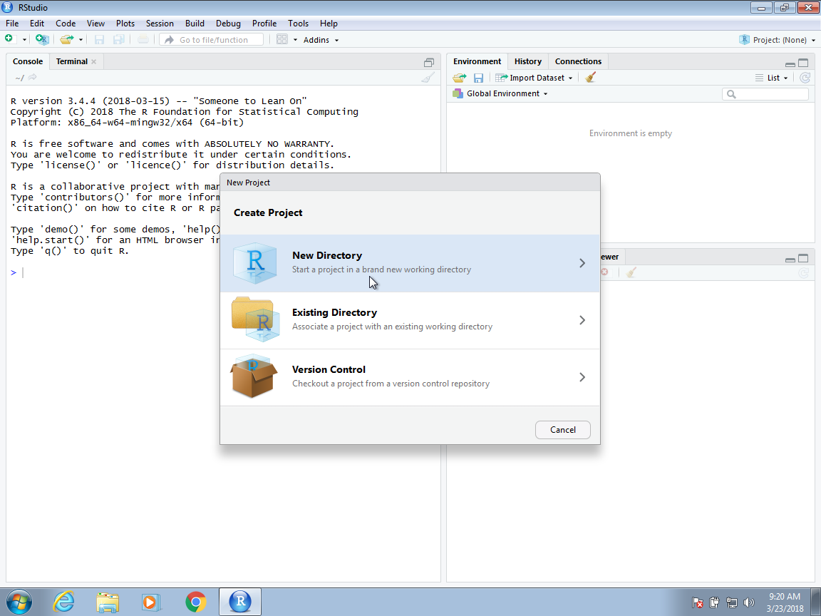
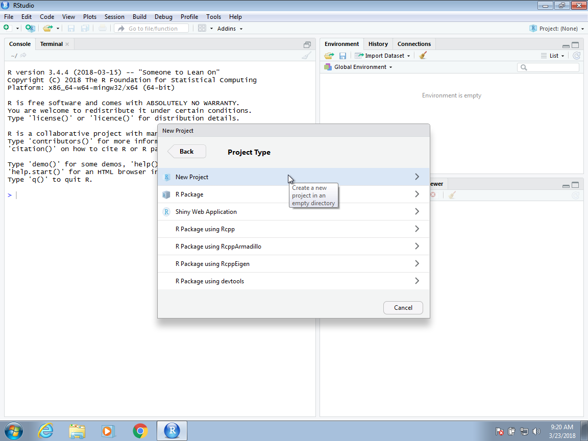
Then, for a data analysis project, you usually select the New Project option:
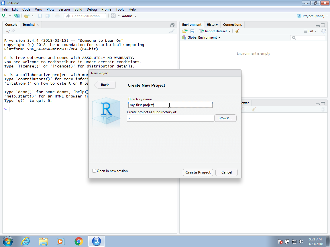
Now you will have to decide on the location of the folder that will be associated with your project, as well as the name of the folder. When choosing a folder name, just like with file names, make sure it is a meaningful name that will help you remember what the project is about. As with files, we recommend using lower case letters, no spaces, and hyphens to separate words. For example, we could call the folder for this project my-first-project. This will then generate a Rproj file called my-first-project.Rproj in the folder associated with the project. We will see how this is useful a few lines below.
You will be given options on where this folder should be on your filesystem. In this example, we will place it in our home My Documents folder, but this is generally not good practice. You want to organize your filesystem following a hierarchical approach. For work associated with this book, you might create separate projects under a common Statistics4Ecologists folder.
One of the main advantages of using Projects is that after closing RStudio, if we wish to continue where we left off on the project, we simply double click or open the file saved when we first created the RStudio project. In this case, the file is called my-first-project.Rproj. If we open this file, RStudio will start up and open any scripts we previously had open from this project.
A.4 R markdown
R markdown is a format for literate programming documents. It is based on markdown, a markup language that is widely used to generate html pages. You can learn more about markdown here: https://www.markdowntutorial.com/. Unlike a word processor, such as Microsoft Word, where what you see is what you get, with R markdown, you need to compile the document into the final report. The R markdown document looks different than the final product. This seems like a disadvantage at first, but it is not because, for example, instead of producing plots and inserting them one by one into the word processing document, the plots are automatically added.
In RStudio, you can start an R markdown document by clicking on File, New File, the R Markdown. You will then be asked to enter a title and author for your document. You can also decide what format you would like the final report to be in: HTML, PDF, or Microsoft Word. Later, we can easily change this, but here we select html as it is the preferred format for debugging purposes and fill in our name and a title:

This will generate a template file:

As a convention, we use the Rmd suffix for these files. In the template, you will see several things to note.
A.4.1 The header
At the top you see:
---
title: "My First Report"
author: "John Fieberg"
date: "2/28/2022"
output: html_document
---
The --- is used to indicate a YAML header. We do not actually need a header, but it is often useful. You can define many other things in the header than what is included in the template (see e.g., the Markdown resources in Section A.5). Also, note that we can change the output parameter to pdf_document (if we have LaTex installed) or word_document if we have MS Word installed. This will change the type of output that is produced when we compile our report.
A.4.2 R code chunks
In various places in the document, we see something like this:
```{r}
summary(pressure)
```
These are the code chunks. When you compile the document, the R code inside the chunk, in this case summary(pressure), will be evaluated and the result included in that position in the final document.
To add your own R chunks, you can type the characters above quickly with the key binding command-option-I on the Mac and Ctrl-Alt-I on Windows.
This applies to plots as well; the plot will be placed in that position. We can write something like this:
```{r}
plot(pressure)
```
By default, the code will show up as well. To avoid having the code show up, you can use an argument. To avoid this, you can use the argument echo=FALSE. For example:
```{r, echo=FALSE}
summary(pressure)
```
We recommend getting into the habit of adding a label to the R code chunks. This will be very useful when debugging, among other situations. You do this by adding a descriptive word like this:
```{r pressure-summary}
summary(pressure)
```
Lastly, note that any errors in your code will prevent you from being able to generate a report to share. One way around this is to add the following code to the top of your .Rmd file:
```{r}
knitr::opts_chunk$set(
  error = TRUE # do not interrupt in case of errors
)
```
A.4.3 Global options
One of the R chunks contains a complex looking call:
```{r setup, include=FALSE}
knitr::opts_chunk$set(echo = TRUE)
```
We will not cover this here, but as you become more experienced with R Markdown, you will learn the advantages of setting global options for the compilation process.
A.4.4 knitR
We use the knitR package to compile R markdown documents. The specific function used to compile is the knit function, which takes a filename as input. RStudio provides a button that makes it easier to compile the document.
The first time you click on the Knit button, a dialog box may appear asking you to install packages you need.
Once you have installed the packages, clicking the Knit will compile your R markdown file and the resulting document will pop up and an html document will be saved in your working directory. To view it, open a terminal and list the files. You can open the file in a browser and use this to present your analysis.
A.5 More on R markdown
There is a lot more you can do with R markdown. We highly recommend you continue learning as you gain more experience writing reports in R. There are many free resources on the internet including:
- RStudio’s tutorial: https://rmarkdown.rstudio.com
- The cheat sheet: https://www.rstudio.com/wp-content/uploads/2015/02/rmarkdown-cheatsheet.pdf
- The knitR book: https://yihui.name/knitr/
- The R Markdown cookbookhttps://bookdown.org/yihui/rmarkdown-cookbook/