Chapter 18 Linear Mixed Effects Models
Learning objectives:
Be able to identify situations when it is appropriate to use a mixed model
Learn how to implement mixed models in R/JAGs for Normally distributed response variables
Be able to describe models and their assumptions using equations and text and match parameters in these equations to estimates in computer output.
18.1 Consequences of violating the independence assumption
A common assumption of all of the models we have fit so far is that our observations are independent. This assumption is unrealistic if we repeatedly record observations on the same sample units (i.e. we have repeated measures); this assumption may also be violated if our observations are measured close in space or close in time. Let’s consider the implications of having non-independent data and also various strategies for accommodating non-Independence using a simple simulated data set from Schwarz, C. J. (2014). Ch 16: Regression with pseudo-replication. In Course Notes for Beginning and Intermediate Statistics. Available at http://www.stat.sfu.ca/~cschwarz/CourseNotes. Retrieved 2015-03-1 and http://people.stat.sfu.ca/~cschwarz/Stat-650/Notes/MyPrograms/Reg-pseudo/Se-Lake/Se-lake.html. These data are contained in the Data4Ecologists package:
library(Data4Ecologists) # for data
library(tidyverse) # for data wrangling
library(gridExtra) # for plotting
library(lme4)  # for fitting random-effects models
library(nlme) # for fitting random-effects models
library(glmmTMB) # for fitting random-effects models
library(here) # for specifying relative paths
library(sjPlot) # for plotting
library(modelsummary) # for creating output tables
library(kableExtra) # for tables
library(ggplot2)# for plotting
library(performance) # for model diagnostics
library(dplyr) # for data wrangling
theme_set(theme_bw())
options(kableExtra.html.bsTable = T)
data(Selake)
head(Selake)
## Lake Log_Water_Se Log_fish_Se
## 1 a -0.30103 0.9665180
## 2 a -0.30103 1.1007171
## 3 a -0.30103 1.3606978
## 4 a -0.30103 1.0993405
## 5 a -0.30103 1.2822712
## 6 b 0.83600 0.9713466The data set contains Selenium concentrations (on the log scale) in a set of 9 lakes and also from a sample of 83 fish from these same lakes. Selenium can leach from coal into surface waters when coal is mined, and therefore, this data set could conceivably have been collected during an environmental review to determine whether Selenium concentrations in nearby lakes are bioaccumulating in fish. We begin by fitting a simple linear regression model to explore the relationship between logged concentrations in the water (Log_Water_Se) and log concentrations in fish (Log_fish_SE), assuming all locations are independent. Below, we plot the regression line overlaid on the observations.
fit.naive <- lm( Log_fish_Se ~ Log_Water_Se, data=Selake)
plot.naive <- ggplot(data=Selake,
    aes(x=Log_Water_Se, y=Log_fish_Se, col=Lake))+
    ggtitle("Se in Fish vs Se Water with linear regression line")+
    xlab("log(Se) in the water\nPoints jittered")+ylab("log(Se) in fish")+
    geom_point(size=3, position=position_jitter(width=0.05))+
    geom_abline(intercept=coef(fit.naive)[1], slope=coef(fit.naive)[2])+
                    theme(legend.position="none")
residplot <- ggplot(broom::augment_columns(fit.naive, Selake),
                    aes(.fitted, .resid, col=Lake)) +
                    geom_point() +
                    geom_smooth() +
                    ggtitle("Residual vs. fitted values") +
                    xlab("Fitted values") +
                    ylab("Residuals")
ggpubr::ggarrange(plot.naive, residplot, ncol=2, common.legend=TRUE, legend="bottom")
## `geom_smooth()` using method = 'loess' and formula 'y ~ x'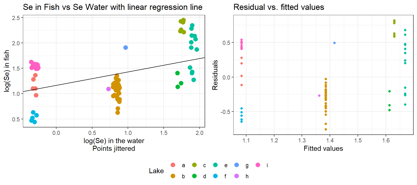
Importantly, the number of fish sampled varies from lake to lake. Further, we see that the residuals for different lakes tend to be clustered with most values being either negative or positive for any given lake. Thus, two randomly chosen residuals from the same lake are likely to be more alike than 2 randomly chosen residuals from different lakes. The data are clearly not independent!
Think-pair-share: What are the consequences of ignoring the fact that we have multiple observations from each lake?
Often when I pose this question to ecologists, they express concern that the estimates of the regression parameters will be biased. Here, it is important to recognize that bias has a specific definition in statistics. In particular, bias is quantified by the difference between the expected (or average) estimate across repeated random trails and the true parameter value. Again, by random trial, we mean the process of collecting and analyzing data in the same way. In this case, that means collecting data in a way that leads to an unbalanced data set (with unequal numbers of fish per lake) and then analyzing that data set using simple linear regression. When our data are not balanced and we treat observations as independent, it is clear that some lakes will contribute more information than others. But, does that imply we have a biased estimator? Well, it depends on the process that leads to the imbalance.
18.1.1 What if sample sizes are random?
Claim: there are clearly other factors that influence Se concentrations in the water and in fish, but if the sample size is completely random (i.e., the number of fish sampled per lake does not depend on these other factors), then our estimates of the regression parameters will be unbiased even if the data set is not balanced. On the other hand, naive estimates of uncertainty will be too small. We can provide support for these claims using simulations.
Let’s use the following data-generation model for log Se concentrations in fish:
\[\begin{gather} log(SeFish)_{i,j} = \beta_0 + \beta_1log(SeWater)_i + \tau_i + \epsilon_{ij} \nonumber \\ \tau_i \sim N(0, \sigma_{\tau}^2) \nonumber \\ \epsilon_{ij} \sim N(0, \sigma_{\epsilon}^2) \nonumber \tag{18.1} \end{gather}\]
where \(log(SeFish)_{i,j}\) is the log Se concentration of the \(j^{th}\) fish in the \(i^{th}\) lake, \(log(SeWater)_i\) is the log Se concentration in \(i^{th}\) lake’s water, and \(\beta_0\) and \(\beta_1\) are the regression parameters we are interested in estimating. Deviations about the regression line are due to two random factors represented by \(\tau_i\) and \(\epsilon_{ij}\); \(\tau_i\) is constant for all observations in a lake whereas \(\epsilon_{ij}\) is unique to each observation. We can think of the \(\tau_i\) as representing factors (other than the Se concentration in a lake) that cause all SeFish concentrations to be higher or lower, on average, for particular lakes56, whereas the \(\epsilon_{ij}\) represent other random factors that create variability among fish found in the same lake. Whenever writing down models for repeated measures data, it is critical that we use multiple subscripts (e.g., we use \(i\) to index each lake and \(j\) to index the different observations within each lake).
We will repeatedly generate a random number of observations from each of 9 lakes using a R’s rnbinom function for generating random values from a negative binomial distribution. We will then fit a linear regression model to the data and store the results to look at the sampling distribution of \(\hat{\beta_0}\), \(\hat{\beta_1}\), \(\widehat{SE}(\hat{\beta}_0)\) and \(\widehat{SE}(\hat{\beta}_1)\):
# Set.seed
set.seed(1024)

# Number of lakes and number of simulations
nlakes <- 10000 # Go Minnesota! :)
nsims <- 10000  # to approximate the sampling distribution

# Parameters used to simulate the data:
beta0 = 1.16 # intercept
beta1 = 0.26 # slope
sigma_tau = 0.45 # sd tau
sigma_epsilon = 0.20 #sd epsilon

# Matrix to hold results
beta.hat <- matrix(NA, nsims, 2)
se.hat <- matrix(NA, nsims, 2)

# Generate lake Se values for each of 10,000 lakes.
# We will assume these are ~N(1,1)
log_se_water<-rnorm(nlakes, 1, 1)

# Generate tau_i for 10,000 lakes
tau <- rnorm(nlakes, 0, sigma_tau)

# Simulation loop
for(i in 1:nsims){
  # pick a sample of 9 lakes
  lakeids <- sample(1:nlakes, 9)

  # determine a random sample size for each lake
  # using a negative binomial random number generator
  # with mean = 9 and overdispersion parameter = 1.15
  ni <- rnbinom(9, mu = 9, size = 1.15)
  log_se_fish <- beta0 + beta1*rep(log_se_water[lakeids], ni) +
                 rep(tau[lakeids], ni) + rnorm(sum(ni), 0, sigma_epsilon)
  dat <- data.frame(id = rep(lakeids, ni),
                    log_se_water = rep(log_se_water[lakeids], ni),
                    log_se_fish)
  lmtemp <- lm(log_se_fish~log_se_water, data=dat)
  beta.hat[i,] <- coef(lmtemp)
  se.hat[i,]<-sqrt(diag(vcov(lmtemp)))
}
Let’s begin by looking at the sampling distributions of our regression parameter estimators with the true parameters used to generate the data highlighted in red:
# plot
par(mfrow=c(1,2))
hist(beta.hat[,1], main="Intercept", xlab="Estimate", ylab="Sampling Distribution")
abline(v=beta0, col="red")
hist(beta.hat[,2], main="Slope", xlab="Estimate", ylab="Sampling Distribution")
abline(v=beta1, col="red")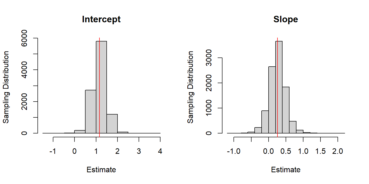
FIGURE 18.1: Sampling distribution for the regression parameter estimators when sample sizes for each lake are random.
There appears to be little bias when estimating \(\beta_0\) and \(\beta_1\) despite having incorrectly assumed the observations were independent, which is also confirmed, below:
## [1] -0.001772321## [1] 0.0004047683Next, we consider the impact that repeated measures have on our estimates of uncertainty when assuming observations are independent. If our estimators of the standard errors of \(\hat{\beta}_0\) and \(\hat{\beta}_1\) are unbiased, then we should expect the average estimated standard errors, \(E[\widehat{SE}(\hat{\beta}_0)]\) and \(E[\widehat{SE}(\hat{\beta}_1)]\), to be close to the standard deviation of \(\hat{\beta}\) (remember, these SEs estimate the standard deviation of our sampling distribution!).
## [1] -0.2411941## [1] -0.1776406We see in both cases that the \(E[\widehat{SE}(\hat{\beta}_i)] < sd(\hat{\beta}_i)\), suggesting our estimates of uncertainty are too small if we ignore the repeated measures and assume our observations are independent.
18.1.2 What if sample sizes are not random?
What if the sample sizes associated with each lake are not random? Maybe we are more likely to sample lakes where fish tend to have high levels of Se (more so than would be predicted by the lake’s Se concentration). I.e., what if the sample sizes were correlated with the \(\tau_i\)? Let’s simulate data under this assumption (but for a sample of 100 lakes) and again fit the simple linear regression model. In addition, we will fit the data-generating model using the lmer function in the lme4 package (Bates, Mächler, Bolker, & Walker, 2015) (this is a mixed-effects model, which will be the subject of the remainder of this Chapter):
# Set.seed
set.seed(1024)

# Matrix to hold results
beta.hat2 <- matrix(NA, nsims, 2)
beta.hat2.lme4 <- matrix(NA, nsims, 2)

# Simulation loop
for(i in 1:nsims){
  # pick a sample of 9 lakes
  lakeids <- sample(1:nlakes, 100)

  # determine random sample size for each lake
  # generate using negative binomial with mean = 9*exp(tau[i])
  # overdispersion parameter = 1.15
  ni <- rnbinom(100, mu = exp(log(9)+tau[lakeids]), size = 1.15)
  log_se_fish <- beta0 + beta1*rep(log_se_water[lakeids], ni) +
    rep(tau[lakeids], ni) + rnorm(sum(ni), 0, sigma_epsilon)
  dat <- data.frame(id = as.factor(rep(lakeids, ni)),
                    log_se_water = rep(log_se_water[lakeids], ni),
                    log_se_fish)
  beta.hat2[i,] <- coef(lm(log_se_fish~log_se_water, data=dat))
  beta.hat2.lme4[i,] <- fixef(lmer(log_se_fish~log_se_water + (1|id), data=dat))
}
We again look at the sampling distributions with the true parameters used to generate the data highlighted in red (the top row of panels correspond to the simple linear regression model and the bottom panels to the mixed-effects model used to generate the data):
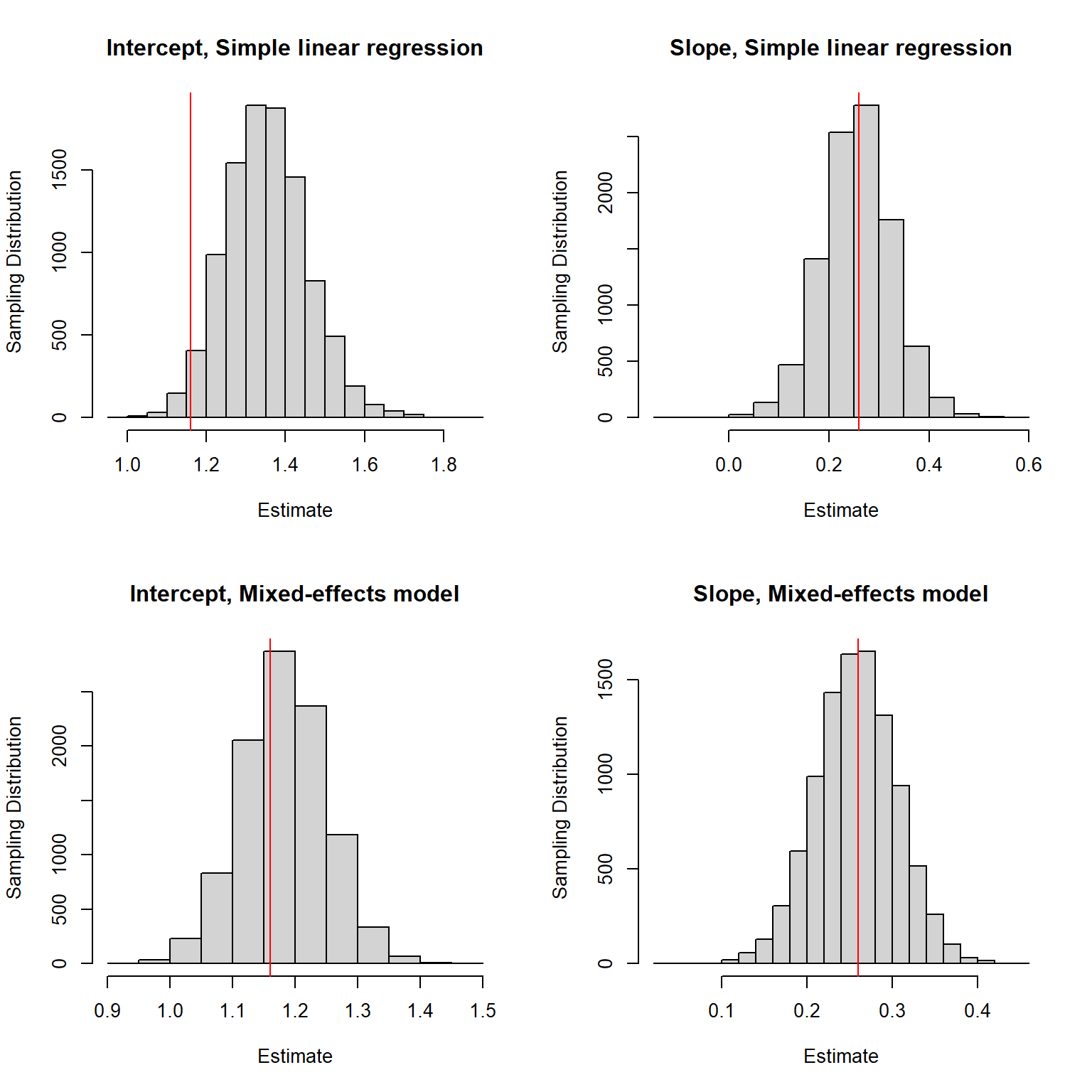
FIGURE 18.2: Sampling distribution for the regression parameter estimators when sample sizes for each lake are correlated with within-lake factors associated with Se concentrations in fish.
We see that when using simple linear regression, our estimator of the intercept is biased. Nonetheless, the estimator of the slope appears to be unbiased. The estimators of both parameters appear to be unbiased when fitting the mixed-effects (i.e., data-generating) model. Also, note that the estimates are less variable when using the mixed-effects model.
bias.betas<-data.frame(
  Method = rep(c("Simple Linear Regression", "Data-Generating (Mixed) Model")),
  Intercept = round(c(mean(beta.hat2[,1])- beta0,
                      mean(beta.hat2.lme4[,1])- beta0), 3),
  Slope = round(c(mean(beta.hat2[,2])- beta1,
                  mean(beta.hat2.lme4[,2])- beta1),3))
bias.betas %>% kable(., caption = "Bias associated with regression parameter estimators.",
booktabs = TRUE)| Method | Intercept | Slope |
|---|---|---|
| Simple Linear Regression | 0.193 | -0.004 |
| Data-Generating (Mixed) Model | 0.023 | -0.002 |
18.2 Optional: Mixed-effect models versus simple alternatives
In the last section, we saw that if sample sizes are random, then our estimates of regression parameters will be unbiased, but estimates of their uncertainty will be too small. Thus, one simple strategy for analyzing repeated measures data in cases where sample sizes can be argued to be completely random or the data are balanced (i.e., contain equal numbers of observations for each cluster) is to assume independence when estimating regression parameters, but then use a method for estimating uncertainty that considers the cluster as the independent unit of replication. For example, in Section 2, we explored a cluster-level bootstrap when analyzing the Rikzdat data (resampling beaches with replacement). Similarly, in Section 20 will learn about Generalized Estimating Equations (GEE) that use robust standard errors calculated by considering variation among independent clusters.
Alternatively, we could consider aggregating our data to the lake level before fitting our regression model. Each lake has a single recorded value of log(Se) in the water. We could calculate the average log(Se) among fish for each lake and then fit a regression model with this average as our response variable. This strategy is often reasonable when the predictors of interest do not vary within a cluster (Murtaugh, 2007). The code below shows how to accomplish this in R.
fishse.avg <- Selake %>% group_by(Lake) %>%
   dplyr::summarize(Log_Water_Se=mean(Log_Water_Se), fish.avg.se=mean(Log_fish_Se))
fit.avg <- lm(fish.avg.se ~ Log_Water_Se, data=fishse.avg)
Lastly, although we have not yet introduced mixed-effect models, we can fit the exact model that was used to generate the data using the following code:
Let’s compare the estimated intercept and slope from these 3 approaches: a naive linear regression model, a regression model fit to lake averages, and the mixed-effect model fit using lmer, which was the model used to generate the data.
modelsummary(list("Naive linear model" = fit.naive,
                  "Linear model fit to averages" = fit.avg,
                  "Mixed-effects model" = fit.mixed),
             gof_omit = ".*", estimate  = "{estimate} ({std.error})", statistic=NULL,
             coef_omit = "SD",
             title="Regression coefficients (SE) from a naive linear regression model
             assuming independence, a regression model fit to lake averages, and a
random-intercept model.")| Naive linear model | Linear model fit to averages | Mixed-effects model | |
|---|---|---|---|
| (Intercept) | 1.164 (0.064) | 1.131 (0.209) | 1.132 (0.209) |
| Log_Water_Se | 0.265 (0.059) | 0.367 (0.181) | 0.366 (0.179) |
We see that the estimated standard errors for \(\beta_0\) and \(\beta_1\) are much narrower in the naive linear model, which is not a surprise since this approach treats the data as though they were independent (Table 18.2). On the other hand, the estimates of \(\beta_0\), \(\beta_1\), and their standard errors are nearly identical when fitting a linear model to the aggregated data or when fitting an appropriate mixed-effects model. An advantage of the former approach is its simplicity – it requires only methods you would likely have seen in an introductory statistics course.
Murtaugh (2007) provided a similar example in which he compared 2 analyses, both aiming to test for differences in mean zooplankton size between ponds that either contained or did not contain fish. In each pond, he measured the body length of thousands of zooplankters. Clearly, these observations will not be independent (zooplankton from the same lake are likely to be more similar to each other than zooplankton from different lakes, even after accounting for the effects of fish presence-absence). The first analysis, reported in Murtaugh (1989), required a full paragraph to describe:
I ran a nested analysis of variance (ANOVA) on the lengths of zooplankton in the six ponds—the effect of pond on body size is nested within the effect of predation treatment. Note that, since the study ponds can be thought of as a sample from a larger population of ponds that might have been used, ‘pond’ is a random effect nested within the fixed effect of fish . . . Because of the complications involved in nested ANOVA’s with unequal sample sizes (Sokal and Rohlf 1981), I fixed the number of replicates per pond at the value for the pond with the smallest number of length measurements available . . .; appropriately-sized samples were obtained from the larger sets of measurements by random sampling without replacement.’’
In the second analysis, he calculated pond-level means and then conducted a two-sample t-test. He points out that the two hypotheses tests relied on the exact same assumptions and the p-values were identical. The nested analysis of variance will sound more impressive, but the latter approach has the advantage of simplicity – again, requiring only methods learned in an introductory statistics class. Murtaugh (2007) makes a strong argument for the simpler analyses, highlighting that:
Simpler analyses are easier to explain and understand; they clarify what the key units in a study are; they reduce the chances for computational mistakes; and they are more likely to lead to the same conclusions when applied by different analysts to the same data.
On the other hand, there are potential advantages of fitting a mixed-effects model (e.g., we will see that we can study variability in Log_Se_fish measurements both among and within lakes). In addition, mixed-effects models will be more powerful when studying predictor-response relationships when the predictor variable varies within a lake. For example, if we also wanted to study how Se concentrations change as fish age, we would be better off studying this using a model that included the age of each fish rather than modeling at the lake level using the average age in each lake as a predictor. Thus, it is important to be able to identify when using a mixed-effects model will be beneficial and when it may be viewed as just statistical machismo.57
The rest of this Chapter will be devoted to mixed-effect models that allow observational units or clusters to have their own parameters. We will learn how to write down a set of equations for mixed models (e.g., eq. (18.1)), match R output to the parameters in these equations, explore the assumptions of the model and how to evaluate them, and discover how these models may or may not properly account for non-independence resulting from having multiple observations on the same sampling unit or cluster.
18.3 What are random effects, mixed-effect models, and when should they be used?
The model fit using the lmer function allowed each lake to have its own intercept. More generally, we can consider models that allow each cluster to have its own intercept and slope parameters. Actually, we already saw how we could allow for cluster-specific parameters in Section 3.
Think-pair-share: using what we learned in Section 3, how could we allow each lake to have its own intercept? And, more generally, how could we allow each lake to have its own set of slope parameters?
We could have included Lake in the model using lm(Log_fish_Se ~ Log_Water_Se + Lake, data=Selake). This would have allowed each lake to have its own intercept. Further, if we had a predictor that varied within a lake (e.g., fish age), we could allow for lake-specific slopes by interacting Lake with age, e.g., using lm(Log_fish_Se ~ Log_Water_Se + age + Lake + age:Lake, data=Selake). These approaches model among-cluster variability using fixed effects, parameters that we directly estimate when fitting the model. How do these parameters differ from random effects?
The defining characteristic of random effects is that they are assumed to come from a common statistical distribution, usually a Normal distribution. Thus, models that contain random effects add another assumption, namely that the cluster-specific parameters come from a common distribution. Specifically, if we examine eq. (18.1), we see the assumption that \(\tau_i \sim N(0, \sigma^2_{\tau})\).
The assumption that the cluster-specific parameters follow a common distribution makes the model hierarchical. Note that most models with random effects also include fixed effects, and are thus referred to as mixed-effects models or mixed models. Thus, we may refer to the model we fit using lmer as:
- a mixed-effects (or mixed model);
- a random-effects model;
- a hierarchical or multi-level model; or
- a random-intercept model.
Mixed-effect models are useful for analyzing data where:
- there are repeated measures on the same sample units (same site, same animal, same lake)
- the data are naturally clustered or hierarchical in nature (e.g., you are collecting data on individuals that live in packs within multiple populations).
- the experimental or sampling design involves replication at multiple levels of hierarchy (e.g. you have a split-plot design with treatments applied to plots and subplots, you have sampled multiple individuals within each of several households)
- you are interested in quantifying variability of a response across different levels of replication (e.g., among and within lakes, among and within sites, etc)
- you want to generalize to a larger population of sample units than just those that you have observed
These latter two points will hopefully become clearer as we proceed through this Section.
18.4 Two-step approach to building a mixed-effects model
It can be useful to consider building hierarchical models in multiple steps. In the first step, we can build models for individual observations within a cluster (referred to as the level-1 model). In the second step, we can model how the cluster-specific parameters from stage 1 vary across clusters (referred to as the level-2 model). We will demonstrate this approach using a data from a study investigating tradeoffs between maximum age of trees and their size in Mountain pines (Pinus montana) in Switzerland (Bigler, 2016). The data, originally downloaded from dryad here, contain data on the (maximum) age and diameter at breast height (dbh) for 160 trees measured at 20 different sites; I have also appended a variable that records the predominate aspect of each site (Aspect). Although a two-step approach to model fitting has some drawbacks, it is a useful pedagogical tool that reinforces the key feature of mixed-effects models, namely that they include cluster-specific parameters that are assumed to arise from a common statistical distribution. A two-step approach can also serve as a useful tool for exploratory data analysis, particularly for data sets that have few clusters but lots of observations per cluster; a good example is wildlife telemetry studies that collect lots of location data on few individuals.
An important consideration when fitting mixed-effects models is whether available predictors vary within a cluster (referred to as level-1 predictors) or they are constant for each cluster (level-2 predictors). In the pines data set, age is a level-1 predictor, whereas Aspsect is a level-2 predictor. We can see this by exploring the relationship between longevity and age at each site, with the points colored by the predominate aspect (which does not vary within a site).
data(pines)
ggplot(pines, aes(age, dbh, col=Aspect)) +
  geom_point()+
  geom_smooth(method="lm", formula = y ~ x) +
  facet_wrap(~site)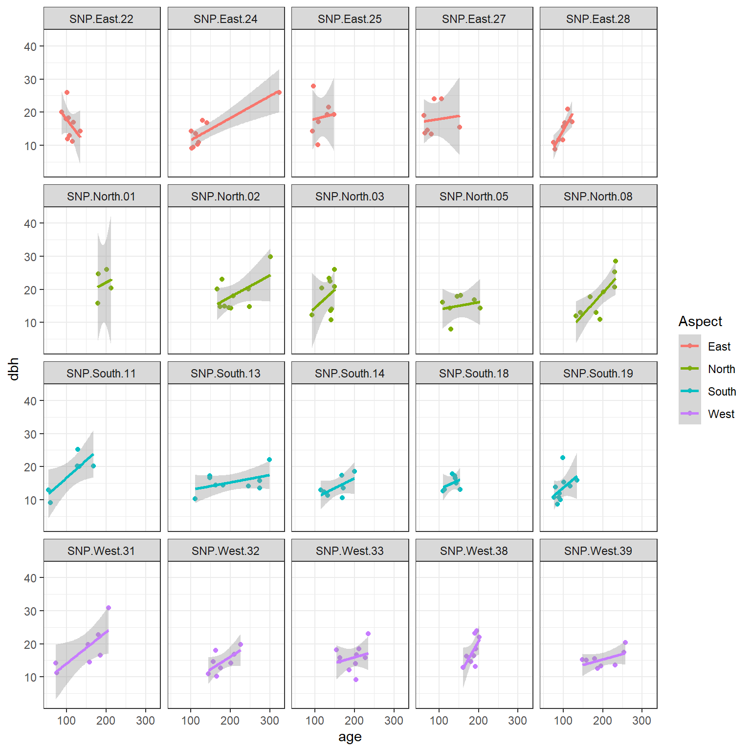
FIGURE 18.3: Diameter at breast height (dbh) versus longevity (age) for 160 pine trees measured at 20 different sites.
We see that the relationship between dbh and age appears to vary by site. We also see that Aspect is constant for all observations from the same site.
18.4.1 Stage 1 (level-1 model)
In the first stage (or step), we build a separate model for each cluster (i.e., site). When building this model, we can only consider variables that are not constant within a cluster. Thus, we can include age but not Aspect.
Level 1 model:
\[\begin{equation} dbh_{ij} = \beta_{0i} + \beta_{1i}age_{ij} + \epsilon_{ij} \tag{18.2} \end{equation}\]
In this model, each site has its own intercept \(\beta_{0i}\) and slope \(\beta_{1i}\). We can use a loop to fit this model to each site, and then pull off the coefficients, or we can accomplish the task in a few lines of code using functions in the purrr (Henry & Wickham, 2020), tidyr (Wickham, 2021), and broom packages (Robinson, Hayes, & Couch, 2021). Before fitting models to each site, we will create a centered and scaled version of age, which will make it easier to fit mixed-effects models down the road (see Section 18.12.2). The scale function creates a new variable, which we name agec, by subtracting the mean age and diving by the standard deviation of age from each observation.
Below, we provide code for fitting a model to each site using a for loop:
usite <- unique(pines$site)
nsites <- length(usite)
Beta <- matrix(NA, nsites, 2) # to hold slope and intercept
Aspect <-  matrix(NA, nsites, 1) # to hold aspect (level- covariate)
for(i in 1:nsites){
  dataseti <- subset(pines, site==usite[i])
  LMi<-lm(dbh~agec, data=dataseti)
  Beta[i,]<-coef(LMi)
  Aspect[i]<-dataseti$Aspect[1]
}
betadat <- data.frame(site = usite,
                      intercept = Beta[,1],
                      slope = Beta[,2],
                      Aspect = Aspect)
betadat
## site intercept slope Aspect
## 1 SNP.South.18 16.097300 2.849878 South
## 2 SNP.North.03 20.309811 5.823510 North
## 3 SNP.East.27 18.953448 1.000244 East
## 4 SNP.North.01 19.069013 3.497746 North
## 5 SNP.North.02 14.697916 3.469895 North
## 6 SNP.East.25 19.580211 1.604887 East
## 7 SNP.North.05 15.136417 1.158623 North
## 8 SNP.South.11 22.318424 5.666733 South
## 9 SNP.West.31 19.140467 5.061144 West
## 10 SNP.West.33 14.366430 1.821074 West
## 11 SNP.South.13 14.189394 1.189321 South
## 12 SNP.South.19 19.034423 5.336379 South
## 13 SNP.East.24 15.108255 3.547825 East
## 14 SNP.South.14 13.727017 3.160221 South
## 15 SNP.East.28 26.010214 11.332107 East
## 16 SNP.West.39 13.760994 1.759141 West
## 17 SNP.West.38 11.105753 11.127715 West
## 18 SNP.West.32 12.578978 4.060440 West
## 19 SNP.East.22 9.500404 -8.309131 East
## 20 SNP.North.08 12.899520 7.010497 NorthAnd, here is an option using functions in the tidyverse set of packages:
betadata <- pines %>% nest_by(site) %>%
  mutate(mod = list(lm(dbh ~ agec, data = data))) %>%
  dplyr::summarize(tidy(mod))
## `summarise()` has grouped output by 'site'. You can override using the `.groups` argument.## Joining, by = "site"## # A tibble: 40 x 7
## # Groups: site [20]
## site term estimate std.error statistic p.value Aspect
## <chr> <chr> <dbl> <dbl> <dbl> <dbl> <chr>
## 1 SNP.East.22 (Intercept) 9.50 5.49 1.73 0.127 East
## 2 SNP.East.22 agec -8.31 6.20 -1.34 0.222 East
## 3 SNP.East.24 (Intercept) 15.1 0.953 15.9 0.000000960 East
## 4 SNP.East.24 agec 3.55 0.747 4.75 0.00209 East
## 5 SNP.East.25 (Intercept) 19.6 4.81 4.07 0.00962 East
## 6 SNP.East.25 agec 1.60 6.25 0.257 0.807 East
## 7 SNP.East.27 (Intercept) 19.0 4.65 4.08 0.00954 East
## 8 SNP.East.27 agec 1.00 3.50 0.286 0.786 East
## 9 SNP.East.28 (Intercept) 26.0 3.25 8.00 0.000203 East
## 10 SNP.East.28 agec 11.3 3.00 3.78 0.00916 East
## # ... with 30 more rows18.4.2 Stage 2 (level-2 model)
In the second step, we treat the coefficients from stage 1 as “data”, and we model the coefficients as a function of variables that are constant within a cluster. Let’s begin by exploring, graphically, how much the coefficients vary across the different sites. We can also see if the coefficients co-vary with our level-2 predictor, Aspect.
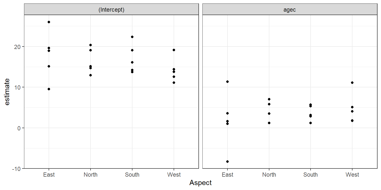
FIGURE 18.4: Distribution of site-specific intercepts and slopes relating longevity to diameter at breast height.
There appears to be quite a bit of site-to-site variability but no strong effect of Aspect on the coefficient estimates. We could also fit regression models relating estimates of cluster-specific parameters to our level-2 predictors (e.g., Aspect). To facilitate further modeling, we will create a “wide” data set containing separate columns for the estimated intercepts and slopes:
betacoefswide <- betadata %>%
  dplyr::select(site, estimate, Aspect, term) %>%
  pivot_wider(names_from = "term", values_from = "estimate") %>%
  rename(intercept = `(Intercept)`, slope = "agec")
We then use this data set to explore how our cluster-specific intercepts and slopes vary and co-vary with our level-2 predictor, Aspect:
##
## Call:
## lm(formula = intercept ~ Aspect, data = betacoefswide)
##
## Residuals:
##     Min      1Q  Median      3Q     Max
## -8.3301 -2.7627 -0.7028  2.1325  8.1797
##
## Coefficients:
##             Estimate Std. Error t value Pr(>|t|)
## (Intercept)  17.8305     1.8569   9.602 4.82e-08 ***
## AspectNorth  -1.4080     2.6260  -0.536    0.599
## AspectSouth  -0.7572     2.6260  -0.288    0.777
## AspectWest   -3.6400     2.6260  -1.386    0.185
## ---
## Signif. codes:  0 '***' 0.001 '**' 0.01 '*' 0.05 '.' 0.1 ' ' 1
##
## Residual standard error: 4.152 on 16 degrees of freedom
## Multiple R-squared:  0.118,  Adjusted R-squared:  -0.04738
## F-statistic: 0.7135 on 3 and 16 DF, p-value: 0.5581##
## Call:
## lm(formula = slope ~ Aspect, data = betacoefswide)
##
## Residuals:
## Min 1Q Median 3Q Max
## -10.1443 -1.2390 -0.5873 1.7001 9.4969
##
## Coefficients:
## Estimate Std. Error t value Pr(>|t|)
## (Intercept) 1.835 1.905 0.964 0.350
## AspectNorth 2.357 2.694 0.875 0.395
## AspectSouth 1.805 2.694 0.670 0.512
## AspectWest 2.931 2.694 1.088 0.293
##
## Residual standard error: 4.259 on 16 degrees of freedom
## Multiple R-squared: 0.07676, Adjusted R-squared: -0.09635
## F-statistic: 0.4434 on 3 and 16 DF, p-value: 0.7252Taken together with Figure 18.4, we might conclude that the coefficients do not vary significantly with respect to Aspect. Thus, we could consider a level-2 model for the site-specific intercepts and slopes that allow these parameters to vary about their overall mean but not depend on Aspect.
Level-2 model:
\[\begin{gather} \beta_{0i} = \beta_0 + b_{0i}\\ \beta_{1i} = \beta_1 + b_{1i} \tag{18.3} \end{gather}\]
In equation (18.3), the \(\beta_0\) and \(\beta_1\) represent the mean intercept and slope in the population of sites, respectively, and \(b_{oi}\) and \(b_{1i}\) represent deviations from these average parameters.
18.4.3 Putting things together: Composite equation
We can combine the level-1 and level-2 models, substituting in the equation for the level-2 model (eq. (18.3)) into the equation for the level-1 model (eq. (18.2)) to form what is referred to as the composite equation:
\[\begin{gather} dbh_{ij} = (\beta_0 +b_{0i}) + (\beta_1+b_{1i})age_{ij} + \epsilon_{ij} \tag{18.4} \end{gather}\]
This leads us to what is referred to as a random coefficient or random slopes model in which both the intercepts and slopes are site-specific. Typically, we also assume that the \((b_{0i}, b_{1i}) \sim N(0,\Sigma_b)\), where \(\Sigma_b\) is a 2 x 2 matrix.
Think-pair-share: why is \(\Sigma_b\) a 2 x 2 matrix? What do the diagonal and non-diagonal entries represent? We will discuss the answer to this question when we explore output from fitting this model in R in Section 18.6.
18.5 Random-intercept versus random intercept and slope model
The 2-step approach of the last section led us to consider a model that included site-specific intercepts and slope parameters associated with our level-1 covariate, agec.58 However, in a great many cases, users default to including only random intercepts without consideration of random slopes59; this choice often leads to p-values that are too small, confidence intervals that are too narrow, and overconfident conclusions when evaluating the importance of level-1 covariates (Schielzeth & Forstmeier, 2009; Arnqvist, 2020; Muff, Signer, & Fieberg, 2020; Silk, Harrison, & Hodgson, 2020). As noted by Schielzeth & Forstmeier (2009), random slopes should generally be considered for predictors that vary within a cluster, especially when cluster-specific parameters exhibit a high degree of variation (Scenario A in Figure 18.5A), when within cluster variability is low (Scenario A in Figure 18.5B), and when there are lots of observations per cluster (Scenario A in Figure 18.5C). In addition to Schielzeth & Forstmeier (2009), Arnqvist (2020) and Silk et al. (2020) also identify this issue as being one that is neglected by all too many users of mixed-effect models.
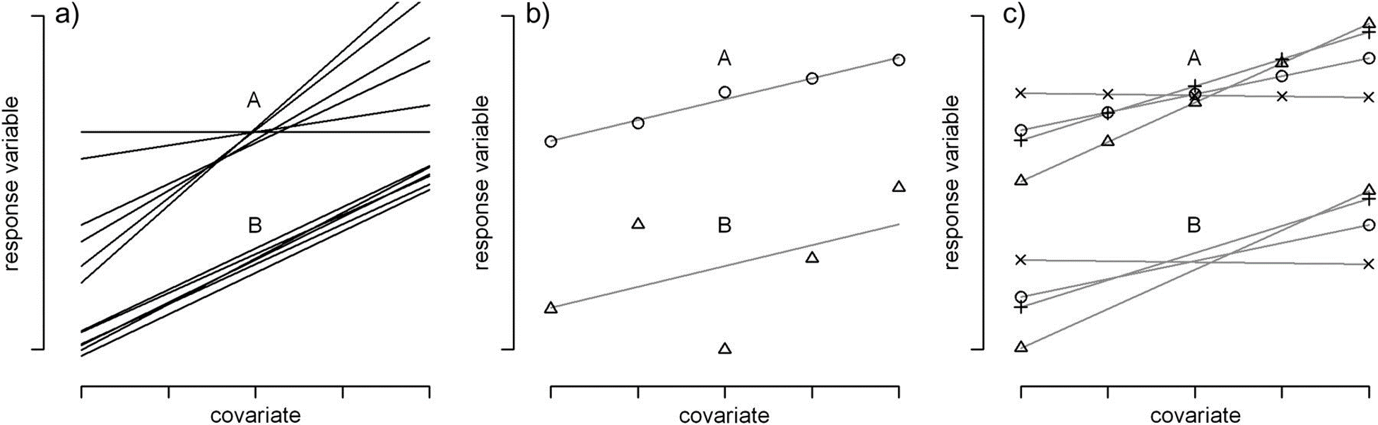
FIGURE 18.5: Figure from Schielzeth & Forstmeier (2009). CC By NC 2.0. Schematic illustrations of more (A) and less (B) problematic cases for the estimation of fixed-effect covariates in random-intercept models. (a) Regression lines for several individuals with high (A) and low (B) between-individual variation in slopes (\(\sigma_b\))). (b) Two individual regression slopes with low (A) and high (B) scatter around the regression line (\(\sigma_r\)). (c) Regression lines with (A) many and (B) few measurements per individual (independent of the number of levels of the covariate).
18.6 Fitting mixed-effects models in R
There are several R packages that can be used to fit mixed-effects models. In this book we will consider 4 of them:
nlme(which only fits linear mixed effects models) (Pinheiro et al., 2021)lme4(Bates et al., 2015)glmmTMB(Brooks et al., 2017)GLMMadaptive(Rizopoulos, 2021) (which only fits generalized linear mixed effect models and not fit linear mixed effect models that use an identity link and assume the distribution of the response is Normal)
We have already seen the nlme package in Section 5, which we used to fit linear models that relaxed the constant variance assumption using generalized least squares. The nlme package is older and less commonly used to fit mixed-effect models than other packages (e.g., lme4 and glmmTMB). The primary advantage of the nlme package is that it can be used to fit mixed models that relax the assumption that within-cluster errors, \(\epsilon_{ij}\), are independent and have constant variance (i.e., one can account for temporal or spatial autocorrelation and non-homogeneous variance). Yet, the nlme package does not include methods for fitting generalized linear mixed effects models (Section 19), and it is slowly becoming outdated. The lme4 package is arguably the most popular package for fitting mixed-effects models, and it will be the focus of this Chapter. The glmmTMB package is newer on the scene and can be quicker for fitting generalized linear mixed effects models (Brooks et al., 2017). It uses similar syntax as lme4 but allows for a wider range of models (e.g., one can fit models that account for zero-inflation, and glmmTMB can also fit mixed-effects models using a negative binomial distribution). Thus, we will explore glmmTMB when we get to Section 19. Lastly, the GLMMadaptive package has certain advantages when fitting generalized linear mixed effects models, particularly when it comes to estimating population-level response patterns. Thus, we will explore this package in Section 19.
For now, we will see how to fit a model with random intercepts and a model with random intercepts and slopes using the lmer function in the lme4 package.
18.6.1 Random intercept model
## Linear mixed model fit by REML ['lmerMod']
## Formula: dbh ~ agec + (1 | site)
## Data: pines
##
## REML criterion at convergence: 918.8
##
## Scaled residuals:
## Min 1Q Median 3Q Max
## -1.9218 -0.7456 -0.0585 0.6020 2.8824
##
## Random effects:
## Groups Name Variance Std.Dev.
## site (Intercept) 4.216 2.053
## Residual 16.147 4.018
## Number of obs: 160, groups: site, 20
##
## Fixed effects:
## Estimate Std. Error t value
## (Intercept) 16.4743 0.5608 29.375
## agec 2.4305 0.4100 5.928
##
## Correlation of Fixed Effects:
## (Intr)
## agec 0.012Think-pair-share: try to describe the model using a set of equations and link the parameters in the equations to the output. We will leave this exercise to the reader but provide this information for the random intercept and slope model below.
18.6.2 Random intercepts and slopes model
## Linear mixed model fit by REML ['lmerMod']
## Formula: dbh ~ agec + (1 + agec | site)
## Data: pines
##
## REML criterion at convergence: 917.4
##
## Scaled residuals:
## Min 1Q Median 3Q Max
## -1.90307 -0.72242 -0.08194 0.58100 2.93686
##
## Random effects:
## Groups Name Variance Std.Dev. Corr
## site (Intercept) 3.740 1.934
## agec 1.122 1.059 0.25
## Residual 15.631 3.954
## Number of obs: 160, groups: site, 20
##
## Fixed effects:
## Estimate Std. Error t value
## (Intercept) 16.5258 0.5601 29.506
## agec 2.4502 0.4934 4.966
##
## Correlation of Fixed Effects:
## (Intr)
## agec 0.157Note, we could have omitted the 1 as lmer by default includes a random intercept whenever a random slope is included. Thus, lmer(dbh ~ agec + (age | site), data = pines) fits the equivalent model as the one above.
Let’s write down this model using a set of equations and find the estimated parameters in the R output:
\[\begin{gather} dbh_{ij} = (\beta_0 +b_{0i}) + (\beta_1+b_{1i})age_{ij} + \epsilon_{ij} \nonumber \\ \epsilon_{ij} \sim N(0, \sigma^2_{\epsilon}) \nonumber \\ \begin{bmatrix} b_{0i}\\ b_{1i} \end{bmatrix} \sim N(\mu, \Sigma_b), \text { with } \tag{18.5} \\ \mu = \begin{bmatrix} 0\\ 0 \end{bmatrix}, \Sigma_b = \begin{bmatrix} \sigma^2_{b_0} & cov(b_0, b_1)\\ cov(b_0, b_1) & \sigma^2_{b1} \end{bmatrix}\\ \end{gather}\]
\(\sigma^2_{b_0}\) is the variance of \(b_{0i}\), \(\sigma^2_{b_1}\) is the variance of \(b_{1i}\), and \(cov(b_0, b_1)= E[b_{0i} b_{1i}] - E[b_{0i}]E[b_{1i}]\) is the covariance of \(b_{0i}\) and \(b_{1i}\). If you are unfamiliar with covariances, they quantify the degree to which two random variables co-vary (i.e., whether high values of \(b_{0i}\) associated with low/high values of \(b_{1i}\)). We can also calculate the covariance from the correlation of two random variables and their standard deviations:
\[\begin{gather} cor(b_0, b_1) = \frac{cov(b_0, b_1)}{\sigma_{b_0}\sigma_{b_1}} \\ \implies cov(b_0, b_1) = cor(b_0, b_1)\sigma_{b_0}\sigma_{b_1} \tag{18.6} \end{gather}\]
The estimates of \(\beta_0\) and \(\beta_1\) are under the label Fixed effects: and are equal to 16.52 and 2.45, respectively. The estimates of \(\sigma^2_{b_0}\), \(\sigma^2_{b_1}\), and \(\sigma^2_{\epsilon}\) are under the label Random effects: and are equal to 3.74, 1.12, and 15.63, respectively. Note that the Std.dev column next to the Variance column just translates these variances to standard deviations (i.e., \(sd(b_1) = \sqrt{\sigma^2_{b_1}} = 1.059\)). The R output from the summary function provides \(cor(b_0, b_1)\) rather than \(cov(b_0, b_1)\). We can calculate \(cov(b_0, b_1)\) using eq. (18.6), \(cov(b_0, b_1) = (0.25)(1.934)(1.059) = 0.512\).
This is a good opportunity to highlight the difference between variability and uncertainty. We describe uncertainty using SEs and confidence intervals. For example, the SE’s for the fixed-effects parameters (Std. Error column) quantify the extent to which our estimates of \(\beta_0\) and \(\beta_1\) would vary across repeated random trials60. Our random intercept and slope model also contains 4 variance/covariance parameters that describe variability in the response variable (within and among sites): \(\sigma^2_{b_0}\), \(\sigma^2_{b_1}\), \(cov(b_0, b_1)\), and \(\sigma^2_{\epsilon}\). It is important to understand that these parameters do not describe uncertainty in the estimated parameters like the SEs do for \(\beta_0\) and \(\beta_1\)!
Think-pair-share: do \(\hat{\sigma}^2_{b_0}\), \(\hat{\sigma}^2_{b_0}\), \(\widehat{cov}(b_0, b_1)\), and \(\hat{\sigma}^2_{\epsilon}\) have sampling distributions?
You bet they do! We estimate these parameters, and therefore, they will have a sampling distribution. We are not given any information here about the uncertainty associated with these parameters, and it turns out that their sampling distribution is usually right skewed. Thus, Normal-based confidence intervals usually do not work well, and SEs do not provide an adequate measure of uncertainty. We can, however,
calculate confidence intervals using the profile-likelihood approach introduced in Section 10.9, which is what the confint function does by default (see below):
## 2.5 % 97.5 %
## .sig01 0.25710190 0.7020577
## .sigma 0.16168696 0.2232918
## (Intercept) 0.72868453 1.5351421
## Log_Water_Se 0.01953563 0.7126375Lastly, note that \(var(\beta_0 + b_{0i}) = var(b_{0i}) = \sigma^2_{b_0}\) because \(\beta_0\) is a constant. Similarly \(var(\beta_1 + b_{1i}) = var(b_{1i}) = \sigma^2_{b_1}\). Thus, we can think of these variance parameters as describing the variance of site-specific deviations from the mean intercept and slope or variability of the site-specific intercepts and slopes themselves.
18.7 Site-specific parameters (BLUPs)
When looking at the output in the last section, you might have wondered why R does not provide estimates of the site-specific parameters – i.e., the intercepts \((\beta_0 +b_{0i})\) and slopes \((\beta_1 +b_{1i})\) for each site. The deviations from the average intercept and slope, \(b_{0i}\) and \(b_{1i}\), are also missing in action. What gives?
In this section, we will learn how to generate “estimates” of site-specific parameters from the mixed-effects model, but we will actually refer to the estimated quantities as “predictions” when fitting models in a frequentist setting – and more specifically, Best Linear Unbiased Predictions (BLUPs) in the context of linear mixed effects models. This distinction arises in frequentist inference because the \(b_{0i}\)’s and \(b_{1i}\)’s are considered to be random variables rather than parameters with fixed but unknown values. If this seems confusing, you are not alone. This is another situation where life just seems easier if you are a Bayesian since all parameters are treated as random variables and assigned probability distributions. There is nothing philosophically different about random effects if you are a Bayesian, other than these parameters will all be assigned a common distribution. We will then need to specify priors for parameters in that common distribution. To see how to implement linear mixed effects models in JAGS, see Section 18.15.
We can generate the BLUPs for \(b_{0i}\) and \(b_{1i}\) in R using the ranef function:
## $site
## (Intercept) agec
## SNP.East.22 1.0581009 -0.539278703
## SNP.East.24 -0.9713254 0.511836750
## SNP.East.25 2.0985073 -0.195316866
## SNP.East.27 1.9471416 -0.659731780
## SNP.East.28 0.4036588 0.341754637
## SNP.North.01 1.5173623 0.510452398
## SNP.North.02 -0.5543028 0.087613361
## SNP.North.03 1.8144629 0.262796638
## SNP.North.05 -0.8777090 -0.282413026
## SNP.North.08 -0.5255991 0.754697359
## SNP.South.11 2.2017430 0.493258625
## SNP.South.13 -1.9043070 -0.960482225
## SNP.South.14 -1.7227241 -0.131886984
## SNP.South.18 -0.3500402 0.005026152
## SNP.South.19 -0.1677626 0.242216046
## SNP.West.31 1.6388877 0.882281861
## SNP.West.32 -1.9592144 -0.291839131
## SNP.West.33 -1.6116716 -0.556945196
## SNP.West.38 -0.1456621 0.214895844
## SNP.West.39 -1.8895462 -0.688935759
##
## with conditional variances for "site"If we want an estimate of uncertainty to accompany the BLUPs, we can use the tidy function in the broom.mixed package (Bolker & Robinson, 2021):
## # A tibble: 40 x 6
## effect group level term estimate std.error
## <chr> <chr> <chr> <chr> <dbl> <dbl>
## 1 ran_vals site SNP.East.22 (Intercept) 1.06 1.31
## 2 ran_vals site SNP.East.24 (Intercept) -0.971 1.10
## 3 ran_vals site SNP.East.25 (Intercept) 2.10 1.32
## 4 ran_vals site SNP.East.27 (Intercept) 1.95 1.45
## 5 ran_vals site SNP.East.28 (Intercept) 0.404 1.40
## 6 ran_vals site SNP.North.01 (Intercept) 1.52 1.36
## 7 ran_vals site SNP.North.02 (Intercept) -0.554 1.14
## 8 ran_vals site SNP.North.03 (Intercept) 1.81 1.15
## 9 ran_vals site SNP.North.05 (Intercept) -0.878 1.18
## 10 ran_vals site SNP.North.08 (Intercept) -0.526 1.11
## # ... with 30 more rowsWe can also easily plot the BLUPs for \(b_{0i}\) and \(b_{1i}\) using the plot_model function in the sjPlot library (Lüdecke, 2021):
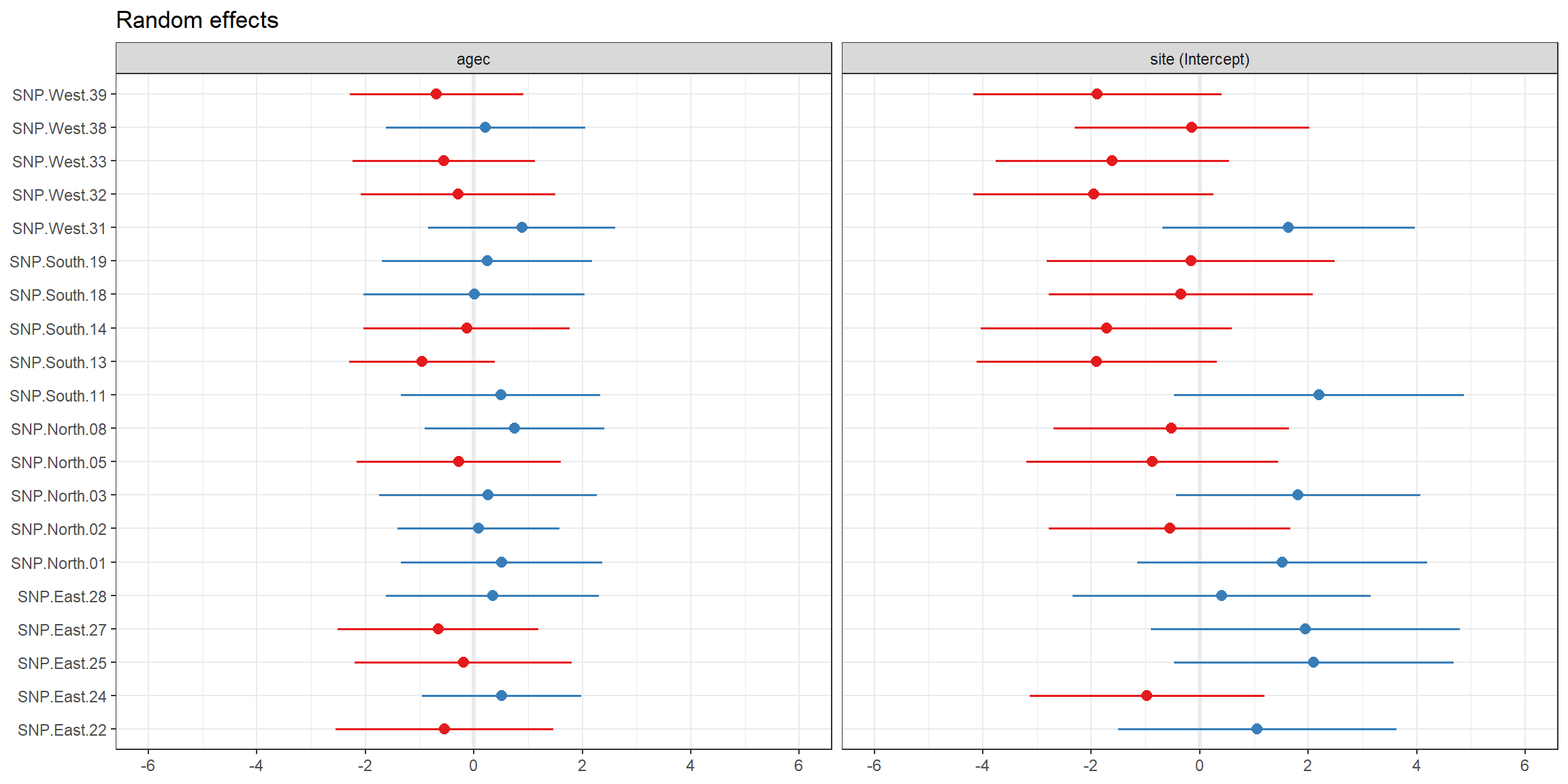
FIGURE 3.8: BLUPs for \(b_{0i}\) and \(b_{1i}\), along with their uncertainty, plotted using the plot_model function in the sjPlot package.
Lastly, we can calculate “estimates” of the cluster-specific parameters by adding \(\hat{\beta}_0\) and \(\hat{\beta}_1\) to the BLUPs for \(b_{0i}\) and \(b_{1i}\). These estimates can also be extracted directly using the coef function:
## $site
## (Intercept) agec
## SNP.East.22 17.58393 1.910931
## SNP.East.24 15.55450 2.962047
## SNP.East.25 18.62434 2.254893
## SNP.East.27 18.47297 1.790478
## SNP.East.28 16.92949 2.791965
## SNP.North.01 18.04319 2.960662
## SNP.North.02 15.97153 2.537823
## SNP.North.03 18.34029 2.713007
## SNP.North.05 15.64812 2.167797
## SNP.North.08 16.00023 3.204907
## SNP.South.11 18.72757 2.943469
## SNP.South.13 14.62152 1.489728
## SNP.South.14 14.80310 2.318323
## SNP.South.18 16.17579 2.455236
## SNP.South.19 16.35807 2.692426
## SNP.West.31 18.16472 3.332492
## SNP.West.32 14.56661 2.158371
## SNP.West.33 14.91416 1.893265
## SNP.West.38 16.38017 2.665106
## SNP.West.39 14.63628 1.761274
##
## attr(,"class")
## [1] "coef.mer"Note, however, that it is not straightforward to calculate uncertainty associated with the cluster-specific intercepts \((\beta_0 +b_{0i})\) and slopes \((\beta_1 +b_{1i})\) as this would require consideration of uncertainty in both \(\hat{\beta}_0, \hat{\beta}_1\) and \(\hat{b}_{0i}, \hat{b}_{1i}\), including how these estimates/predictions co-vary (see this link on Ben Bolker’s GLMM FAQ page).
18.7.1 Digging deeper, how are the BLUPS calculated?
To understand how how BLUPS are calculated from a fitted mixed-effects model, it is helpful to write the model down in terms of the conditional distribution of \(Y\) given the random effects (i.e., \(f_{Y | b}(y)\)) and the distribution of the random effects, \(f_b(b)\). This way of writing down the model also makes it easy to generalize to other types of probability distributions (i.e., generalized linear mixed effect models), which we will see in Section 19.
We can describe our random intercept and slope model from the last section as:
\[\begin{gather} dbh_{ij} | b_{0i}, b_{1i} \sim N(\mu_i, \sigma^2_{\epsilon}) \tag{18.7} \\ \mu_{ij} = (\beta_0 +b_{0i}) + (\beta_1+b_{1i})age_{ij} \nonumber \\ \begin{bmatrix} b_{0i}\\ b_{1i} \end{bmatrix} \sim N(0, \Sigma_b), \text { with} \tag{18.8} \\ \Sigma_b = \begin{bmatrix} \sigma^2_{b_0} & cov(b_0, b_1)\\ cov(b_0, b_1) & \sigma^2_{b1} \end{bmatrix} \end{gather}\]
And, more generally, we can write down any linear mixed effects model using:
\[\begin{gather} Y_{ij} \mid b \sim N(\mu_i, \sigma^2_{\epsilon}) \nonumber \\ \mu_{ij} = X\beta + Zb \\ b \sim N(0, \Sigma_b) \nonumber \end{gather}\]
Here, \(Z\) is a design matrix associated with the random effects. For a random-intercept model, Z would contain a column of 1’s. For our random intercept and slope model, \(Z\) would also contain a column with the values of agec.
The BLUPs, which are returned by the ranef function, are estimated by maximizing:
\[\begin{gather} f_{b|Y}(b) = \frac{f_{Y|b}(y)f_b(b)}{f_Y(y)} \end{gather}\]
where \(f_{b|Y}(b)\) is the posterior distribution of the random effects given the observed data, \(f_b(b)\) is the distribution of the random effects (given by eq. (18.8)), and \(f_{Y|b}(y)\) is the conditional distribution of \(Y |b\) (given by eq. (18.7)). The BLUPs are often referred to as conditional modes and have a Bayesian flavor to them. To calculate the BLUPs, we have to substitute in the estimated fixed effects and variance parameters into our equations for \(f_{Y|b}(y)\) and \(f_b(b)\), leading to what is sometimes referred to as an Empirical Bayes estimator.
18.8 Fixed versus random effects and shrinkage
Earlier, I hinted at the fact that we could estimate site-specific intercepts and slopes using a linear model without random effects. Let’s go ahead and fit a fully fixed-effects model and compare our results to those from the mixed model:
##
## Call:
## lm(formula = dbh ~ site + agec + site:agec, data = pines)
##
## Residuals:
## Min 1Q Median 3Q Max
## -8.1059 -2.3715 -0.0893 2.0420 9.9533
##
## Coefficients:
## Estimate Std. Error t value Pr(>|t|)
## (Intercept) 9.500 4.879 1.947 0.05383 .
## siteSNP.East.24 5.608 5.059 1.109 0.26985
## siteSNP.East.25 10.080 5.791 1.741 0.08430 .
## siteSNP.East.27 9.453 6.058 1.561 0.12127
## siteSNP.East.28 16.510 7.246 2.279 0.02446 *
## siteSNP.North.01 9.569 7.653 1.250 0.21361
## siteSNP.North.02 5.198 5.340 0.973 0.33233
## siteSNP.North.03 10.809 5.262 2.054 0.04212 *
## siteSNP.North.05 5.636 5.100 1.105 0.27137
## siteSNP.North.08 3.399 5.238 0.649 0.51762
## siteSNP.South.11 12.818 5.386 2.380 0.01890 *
## siteSNP.South.13 4.689 5.159 0.909 0.36524
## siteSNP.South.14 4.227 5.100 0.829 0.40889
## siteSNP.South.18 6.597 5.472 1.206 0.23038
## siteSNP.South.19 9.534 6.542 1.457 0.14760
## siteSNP.West.31 9.640 5.103 1.889 0.06128 .
## siteSNP.West.32 3.079 5.265 0.585 0.55980
## siteSNP.West.33 4.866 5.412 0.899 0.37040
## siteSNP.West.38 1.605 6.096 0.263 0.79273
## siteSNP.West.39 4.261 5.354 0.796 0.42775
## agec -8.309 5.500 -1.511 0.13351
## siteSNP.East.24:agec 11.857 5.600 2.117 0.03629 *
## siteSNP.East.25:agec 9.914 6.832 1.451 0.14933
## siteSNP.East.27:agec 9.309 6.129 1.519 0.13142
## siteSNP.East.28:agec 19.641 7.393 2.657 0.00897 **
## siteSNP.North.01:agec 11.807 9.197 1.284 0.20170
## siteSNP.North.02:agec 11.779 5.741 2.052 0.04238 *
## siteSNP.North.03:agec 14.133 6.835 2.068 0.04081 *
## siteSNP.North.05:agec 9.468 6.039 1.568 0.11955
## siteSNP.North.08:agec 15.320 5.845 2.621 0.00990 **
## siteSNP.South.11:agec 13.976 5.882 2.376 0.01909 *
## siteSNP.South.13:agec 9.498 5.605 1.695 0.09272 .
## siteSNP.South.14:agec 11.469 6.147 1.866 0.06450 .
## siteSNP.South.18:agec 11.159 7.677 1.454 0.14866
## siteSNP.South.19:agec 13.646 6.767 2.016 0.04600 *
## siteSNP.West.31:agec 13.370 5.730 2.333 0.02129 *
## siteSNP.West.32:agec 12.370 6.156 2.009 0.04674 *
## siteSNP.West.33:agec 10.130 6.046 1.676 0.09641 .
## siteSNP.West.38:agec 19.437 7.852 2.475 0.01470 *
## siteSNP.West.39:agec 10.068 5.817 1.731 0.08607 .
## ---
## Signif. codes: 0 '***' 0.001 '**' 0.01 '*' 0.05 '.' 0.1 ' ' 1
##
## Residual standard error: 3.93 on 120 degrees of freedom
## Multiple R-squared: 0.4727, Adjusted R-squared: 0.3013
## F-statistic: 2.758 on 39 and 120 DF, p-value: 1.301e-05This model gives us direct estimates of intercepts and slopes for each site along with their uncertainty. If we are predominately interested in these particular sites, then this model is much more straightforward to work with (e.g., we do not have to try to understand what BLUPs are!). On the other hand, this model requires fitting a lot of parameters (40 in total) and it does not allow us to generalize to other sites that we may not have sampled. In addition, we are unable to consider level-2 predictors in this model since they will be confounded with the site-specific intercepts (to see this, we can try adding Aspect to the model, which will result in NA for several of the coefficient estimates):
## (Intercept) siteSNP.East.24 siteSNP.East.25
## 9.500404 5.607851 10.079807
## siteSNP.East.27 siteSNP.East.28 siteSNP.North.01
## 9.453044 16.509810 9.568609
## siteSNP.North.02 siteSNP.North.03 siteSNP.North.05
## 5.197512 10.809407 5.636013
## siteSNP.North.08 siteSNP.South.11 siteSNP.South.13
## 3.399116 12.818020 4.688990
## siteSNP.South.14 siteSNP.South.18 siteSNP.South.19
## 4.226613 6.596896 9.534019
## siteSNP.West.31 siteSNP.West.32 siteSNP.West.33
## 9.640063 3.078574 4.866026
## siteSNP.West.38 siteSNP.West.39 agec
## 1.605349 4.260590 -8.309131
## AspectNorth AspectSouth AspectWest
## NA NA NA
## siteSNP.East.24:agec siteSNP.East.25:agec siteSNP.East.27:agec
## 11.856956 9.914018 9.309375
## siteSNP.East.28:agec siteSNP.North.01:agec siteSNP.North.02:agec
## 19.641238 11.806878 11.779026
## siteSNP.North.03:agec siteSNP.North.05:agec siteSNP.North.08:agec
## 14.132642 9.467754 15.319628
## siteSNP.South.11:agec siteSNP.South.13:agec siteSNP.South.14:agec
## 13.975865 9.498452 11.469352
## siteSNP.South.18:agec siteSNP.South.19:agec siteSNP.West.31:agec
## 11.159010 13.645510 13.370275
## siteSNP.West.32:agec siteSNP.West.33:agec siteSNP.West.38:agec
## 12.369572 10.130205 19.436846
## siteSNP.West.39:agec
## 10.068272Otherwise, how do our estimates of site-specific parameters from the fixed-effect model compare to the BLUPs from the mixed-effect model? Lets plot them together to see! To facilitate comparison, we will refit our fixed effects model using means coding. Then, we create a data set with the coefficients from both models for plotting.
lmmeans.fc <- lm(dbh ~ site + agec + site:agec -1 - agec, data=pines)
coef.fixed <- coef(lmmeans.fc)
coef.random <- coef(lmer.rc)$site
coefdat <- data.frame(intercepts = c(coef.fixed[1:20], coef.random[,1]),
slopes = c(coef.fixed[21:40], coef.random[,2]),
method = rep(c("Fixed", "Random"), each=20),
site = rep(names(coef.fixed)[1:20],2))Figure 18.6 compares the estimates of site-specific intercept and slope parameters from the fixed-effects and mixed-effects models. The estimated mean intercept (\(\hat{\beta}_0\)) and slope (\(\hat{\beta}_1\)) in the population of sites is also depicted by a black horizontal line.
p1 <- ggplot(coefdat, aes(site, intercepts, col=method)) +
geom_point(size=2)+ ggtitle("Intercepts")+
theme(axis.text.x = element_text(angle = 45, hjust = 1)) +
geom_hline(yintercept=summary(lmer.rc)$coef[1,1])
p2 <- ggplot(coefdat, aes(site, slopes, col=method)) +
geom_point(size=2)+ ggtitle("Slopes")+
theme(axis.text.x = element_text(angle = 45, hjust = 1)) +
geom_hline(yintercept=summary(lmer.rc)$coef[2,1])
ggpubr::ggarrange(p1, p2, ncol=2, common.legend=TRUE, legend="bottom") 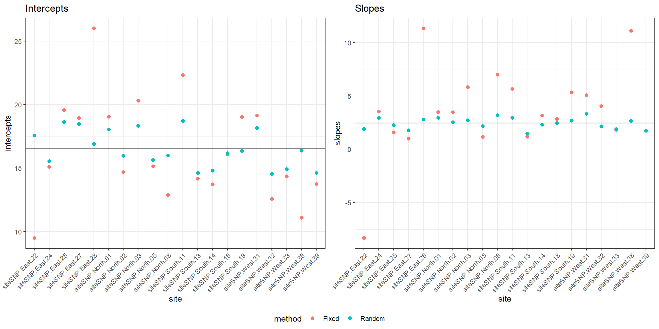
FIGURE 18.6: Comparison of fixed versus random effects parameters demonstrating the shrinkage property of random-effects.
Alternatively, we could compare the two sets of coefficients by plotting the (intercept, slope) pairs and connecting them for the two methods (Figure 18.7).
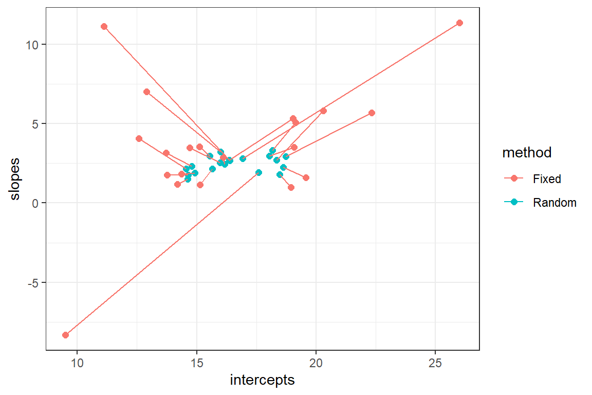
FIGURE 18.7: Comparison of fixed versus random effects parameters demonstrating the shrinkage property of random-effects.
We see that the coefficients for the random effects are shrunk back towards the estimated mean coefficients in the population (\(\hat{\beta}_0\) and \(\hat{\beta}_1\)). The degree of shrinkage depends on the amount of information available for each site and also on the relative magnitude of the variance among sites (\(\hat{\sigma}^2_{b_0}, \hat{\sigma}^2_{b_1}\)) relative to the variance within sites (\(\hat{\sigma}^2_{\epsilon}\)). Coefficients for sites that have few observations and that lie far from the population mean will exhibit more shrinkage than those with more observations and that lie closer to the population mean. Coefficients will also exhibit more shrinkage in applications where the within-site variability is large relative to the total (within- plus among-site) variability.
Recall that what makes random effects different from fixed effects is that we assume our random-effect parameters all come from a common distribution. If parameters come from a common distribution, then it makes sense to “borrow information” from other sites when estimating site-specific parameters. The extent to which information from other sites is relevant depends on how similar sites are to each other (i.e., the among-site variance). And the value of using other information from other sites increases in cases where the information content from within-site observations is low. Thus, mixed-effect models provide a sensible way to weight information coming from within and among sites.
18.9 Fitted/predicted values from mixed-effects models
Now that we have explored how to estimate (or predict) site-specific parameters, we may also consider two types of predictions when fitting mixed-effect models. Specifically, we may be interested in exploring predictor-response relationships within specific sites or within the population (averaging across different sites). These two types of predictions are often referred to as subject-specific and population-averaged response patterns (e.g., Fieberg, Rieger, Zicus, & Schildcrout, 2009) or conditional and marginal response patterns, respectively (Muff, Held, & Keller, 2016).
Subject-specific mean response patterns (associated with each sampled site):
- \(E[dbh | age, b_{0i}, b_{1i}] = (\beta_0 + b_{0i}) + (\beta_1 + b_{1i})age_{ij}\)
Population-averaged mean response patterns (associated with the population of sites):
- \(E[dbh | age] = E(E[dbh | X, b_{0i}, b_{1i}])) = \beta_0 + \beta_1age\)
We can generate these two types of predictions using the predict function. By default, this will return subject-specific responses: \(\widehat{dbh}_{ij} = (\hat{\beta}_0 + \hat{b}_{0i}) + (\hat{\beta}_1 + \hat{b}_{1i})age_{ij}\). Below, we compare site-specific response patterns from the mixed-effects model (red) to those obtained from the fixed-effects model (blue).
# Subject-specific regression lines from the mixed-effects model
pines$sspred.rc<-predict(lmer.rc)
# Subject-specific regression lines from the fixed-effects model
pines$fepred<-predict(lmmeans.fc)
# Plot
ggplot(pines, aes(age, dbh)) +
geom_point(size = 2) +
geom_line(aes(age, sspred.rc), lwd = 1.3, col = "red") +
geom_line(aes(age, fepred), lwd = 1.3, col = "blue") +
facet_wrap( ~ site)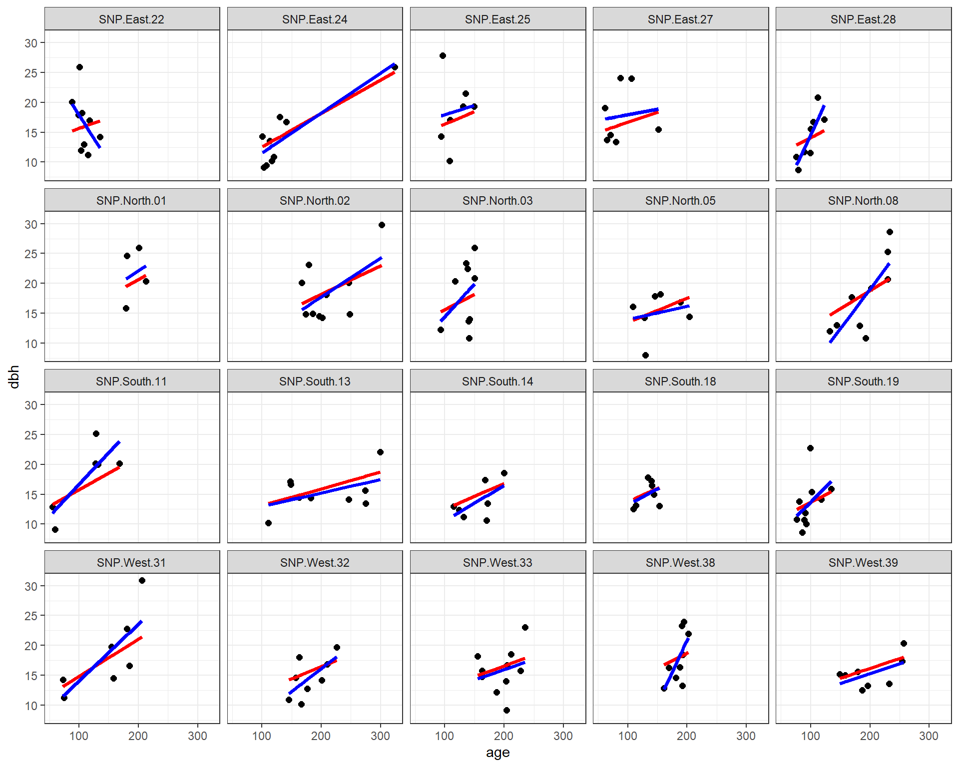
FIGURE 18.8: Fitted regression lines relating dbh to tree age using a fixed - effects (only) model and a model using random intercepts and slopes.
We see that the most of the fitted lines are similar between the two approaches (fixed-effects only and mixed-effects model). However, the estimated slope for SNP.East.22 (upper left corner) was negative when estimated from the fixed effects model and positive when estimated from the mixed-effects model. This result again demonstrates how random effects “borrow information” across sites. The mixed-effects model assumes that all of the slope parameters come from a common distribution. In the fixed-effects model, all of the other slope estimates were positive, and site SNP.East.22 had a limited range of observed ages. Thus, the mixed-effect model infers that the slope for this site should look like the others and should be positive.
What if we had only included random intercepts, as many ecologists tend to do, or fit a fixed-effect model without the interaction between site and agec? Let’s create a similar plot, but this time comparing the random intercept (only) model to the model containing both random intercepts and random slopes.
# Subject-specific lines from random intercept mixed-effects model
pines$sspred.ri <- predict(lmer.ri)
# Subject-specific regression lines from the fixed-effects model
pines$fpred2<-predict(lm(dbh ~ site + agec, data = pines))
# Plot
ggplot(pines, aes(age, dbh)) +
geom_point(size = 2) +
geom_line(aes(age, sspred.ri), lwd = 1.3, col = "red") +
geom_line(aes(age, fpred2), lwd = 1.3, col = "blue") +
facet_wrap( ~ site)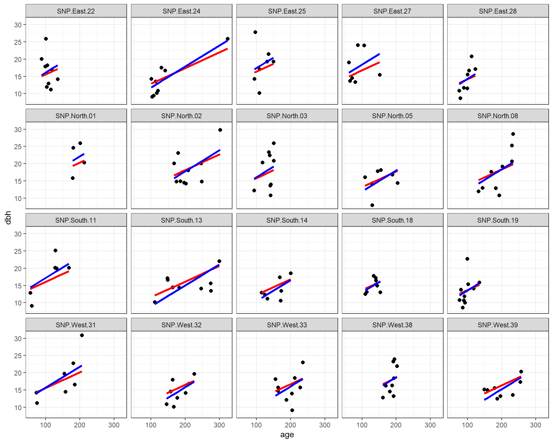
FIGURE 18.9: Fitted regression lines relating dbh to tree age using a fixed-effects (only) model and a mixed-effects model with random intercepts. In both cases, the effect of age is assumed to be constant across sites.
We see that both methods assume the effect of age is constant for all sites, but that each site has its own intercept. The slope parameters are similar for the two methods, but not identical. In addition, the intercepts differ in many cases due to the shrinkage noted previously.
We can also use the predict function to generate population-averaged response curves by supplying an extra argument, re.form = ~ 0, or equivalently, re.form = ~ NA.61
pines$papred <- predict(lmer.rc, re.form = ~0)
ggplot(pines, aes(age, dbh, col=site)) +
geom_point(size=2)+
geom_line(aes(age, papred), lwd=1.3, col="red")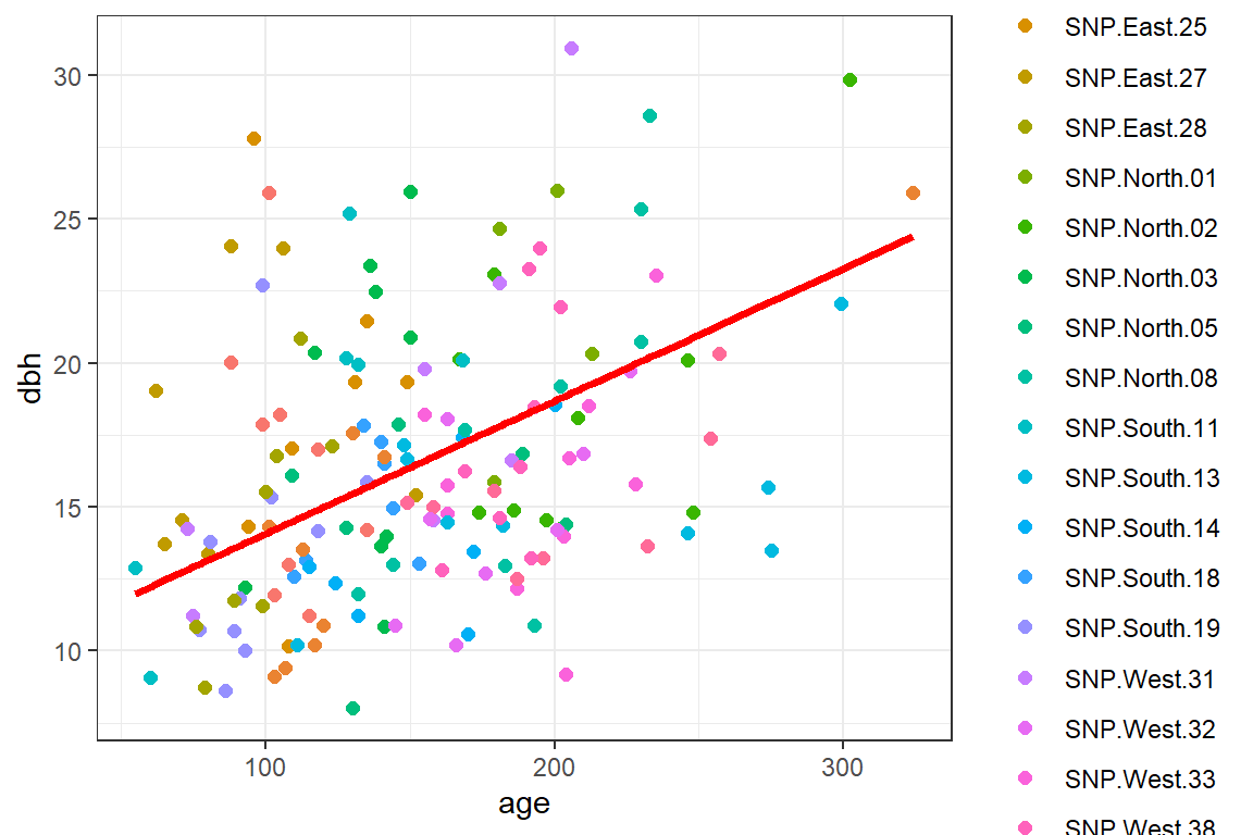
FIGURE 18.10: Population-averaged regression line relating dbh to longevity using a mixed model containing random intercepts and slopes.
The predict function can also be used to generate predictions for new data. Note, however, that when generating subject-specific predictions, the data associated with the newdat argument must include columns corresponding to all of the grouping variables used to specify the random effects in the model (in this case, site).
If you look at the help page for predict.merMod62, you will see that it states:
There is no option for computing standard errors of predictions because it is difficult to define an efficient method that incorporates uncertainty in the variance parameters; we recommend
bootMerfor this task.
We illustrate the use of the bootMer function to calculate uncertainty in our subject-specific predictions, below:
The bootMer function will store the bootstrap statistics (i.e., our predictions for each observation) in a matrix named t:
## [1] 500 160## [1] 160We see that each row contains a different bootstrap statistic for each of the observations in our data set, represented by the different columns. We can use the apply function to calculate quantiles of the bootstrap distribution for each observation, allowing us to construct 95% confidence intervals for the site-specific response patterns:
We then append these values to our pines data set.
Then, we re-create our plot with the site-specific predictions:
# Plot
ggplot(pines, aes(age, dbh)) +
geom_point(size=2)+
geom_line(aes(age, sspred.rc), lwd=1.3, col="red") +
geom_line(aes(age, lowCI), lwd=1.3, col="red", lty=2) +
geom_line(aes(age, upCI), lwd=1.3, col="red", lty=2) +
facet_wrap(~site)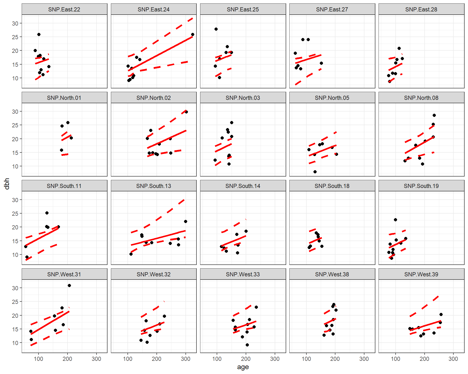
FIGURE 18.11: Fitted regression lines relating dbh to tree age using a mixed model containing random intercepts and slopes. A bootstrap was used to calculate pointwise 95-percent confidence intervals.
One thing that sticks out in Figure 18.11 is that the point estimates do not always fall in the middle of the confidence interval for many of the sites. Recall that the mixed-effects models borrow information across sites. Like other statistical methods that borrow information by smoothing (e.g., generalized additive models, kernel density estimators), or induce shrinkage (e.g., the LASSO estimator from Section 8.6), the subject-specific predictions from the mixed-effects model trade off some level of bias to increase precision. This property makes it challenging to calculate proper confidence intervals for quantities that are a function of \(\hat{b}_{0i}, \hat{b}_{1i}\). If you inspect the boot.pred object we created, you will see that bootMer returns several non-zero estimates of bias associated with the subject-specific predictions.
18.10 Model assumptions
The assumptions of our mixed-effects model are similar to those of linear regression, except we have added another assumption that our random-effects come from a common Normal distribution. Below, we write these assumptions for the random intercept and slopes model; assumptions for the random intercept model can be inferred by setting \(b_{1i}\) to 0.
- Constant within-cluster variance: the within-cluster errors, \(\epsilon_{ij}\), have constant variance (i.e., there is constant scatter about the regression line for each cluster); \(var(\epsilon_{ij}) = \sigma^2_{\epsilon}\)
- Independence: within-cluster errors, \(\epsilon_{ij}\), are independent (both within clusters and across clusters). We also assume the within-cluster errors, \(\epsilon_{ij}\) are independent of the random effects, \((b_{0i}, b_{1i})\).
- Linearity: we may state this assumption in terms of the mean response pattern for a particular site, \(E[Y_i \mid X_i, b_{0i}, b_{1i}] = (\beta_0+ b_{0,i})+ (\beta_1+b_{1i})X_i\), or for the mean response pattern averaged across sites, \(E[Y_i \mid X_i] = \beta_0 + \beta_1X_i\) (see Section 18.9). We can derive the latter expression by noting that \(E[b_{0i}] = E[b_{1i}] = 0\).
- Normality: the \(\epsilon_{ij}\) follow a Normal (Gaussian) distribution; in addition, the random effects, \((b_{0i}, b_{1i})\) are normally distributed: \((b_{0i}, b_{1i}) \sim N(0, \Sigma_b)\)
We can evaluate these assumptions using similar methods to those used to evaluate the assumptions of linear regression (Section 1.4):
- residual versus fitted values plots to evaluate the linearity and constant variance assumptions
- qqplots or histograms/density plots to evaluate assumptions of normality
18.10.1 Evaluating assumptions
Their is a built-in plot function that works with mixed-effect models fit using lme or lmer. This function plots residuals versus subject-specific fitted values, which we explore below for the random-intercept and random intercept and slope models.
ri<-plot(lmer.ri, main = "Random intercept") # residual versus fitted
rc<-plot(lmer.rc, main = "Random intercept and slope")
grid.arrange(ri, rc, ncol=2)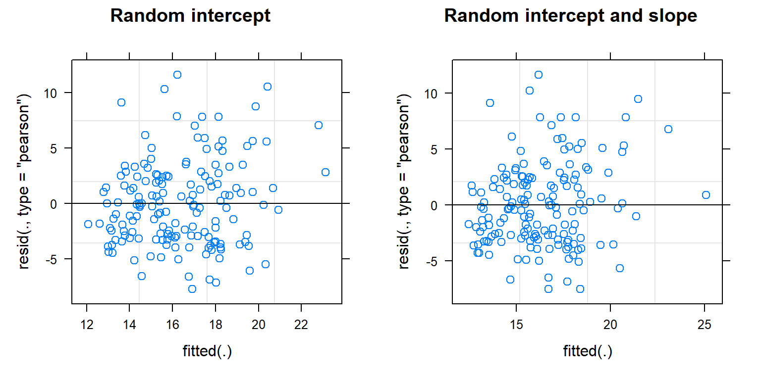
FIGURE 18.12: Residual versus fitted value plots for evaluating linearity and constant variance for the random intercept and random intercept and slope models fit to the pines data.
As with linear regression, we are looking to see whether the residuals have constant scatter as we move from left to right and that there are no trends that would indicate a missing predictor or the need to allow for a non-linear relationship with one of the predictors. These plots do not look too bad, although it looks like the variance may increase some with fitted values
We can evaluate the Normality assumption for the \(\epsilon_{ij}\) and for the random effects using qqplots. The check_model function in the performance package (Lüdecke et al., 2021) will produce these plots, along with standard residual plots used to evaluate linearity and constant variance assumptions of linear regression (Figures 18.13, 18.14).
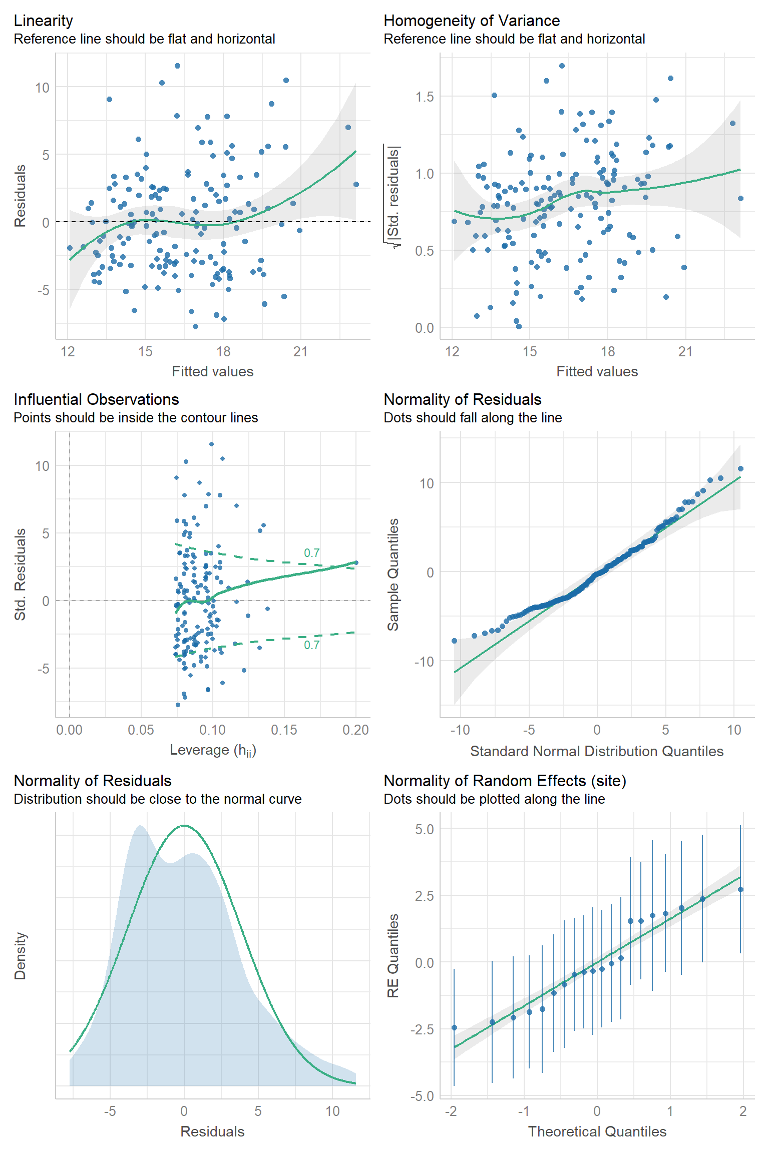
FIGURE 18.13: Residual diagnostic plots using the check_model function in the performance package (Lüdecke et al., 2021) for the random intercept model fit to the pines data set.
The top-left plot is our standard residual versus fitted value plot (the same one that we saw with the default plot method applied to our linear model object). Except for a few outlying points near the extreme left and right of the plot which cause the smooth (green) line to deviate from a horizontal line at 0, the residuals appear to have constant scatter and very little trend. Thus, the linearity assumption seems reasonable. The top-right plot is the scale-location plot that we encountered previously for linear regression models in Section 1.4. Here, we are looking for the locations to have similar mean and variance throughout (and a flat smooth line), indicating the residuals have constant variability. There may be a slight increase in variance for larger fitted values, but overall, this plot doesn’t look too bad to me. The middle-left plot shows standardized residuals plotted against leverage; observations with high values for leverage have predictor values that fall far from the sample mean of the predictor values and are potentially influential observations. We have largely ignored this plot when discussing linear models, but we might consider looking into the points that fall outside the green dotted lines to see if they are in error or if dropping them substantially changes our estimates. Of particular concern would observations that have large residuals and high leverage (i.e., points in the upper or lower right corners of the plot). The next two plots are used to examine the Normality assumption of the within-group errors, \(\epsilon_{ij}\). There are some larger-than-expected residuals that fall far from the line in the QQ-plot (middle-right plot), but these observations largely fall with in the simulation bounds. The distribution of the residuals also appears to have two modes and is not fully symmetric (bottom-left plot), suggesting a slight deviation from the Normality assumption of the within group errors. Lastly, the lower-right plot can be used to evaluate whether the random intercepts are Normally distributed. We see that there are a few sites with intercepts that fall off the QQ-line, but the individual estimates have a lot of uncertainty, with confidence intervals that overlap the QQ-line.
Below, we create the same set of plots for the random intercept and slope model. In this case, we get one more QQ-plot for the random slopes (lower-right plot). Otherwise, the plots look similar to those from the random intercept model.
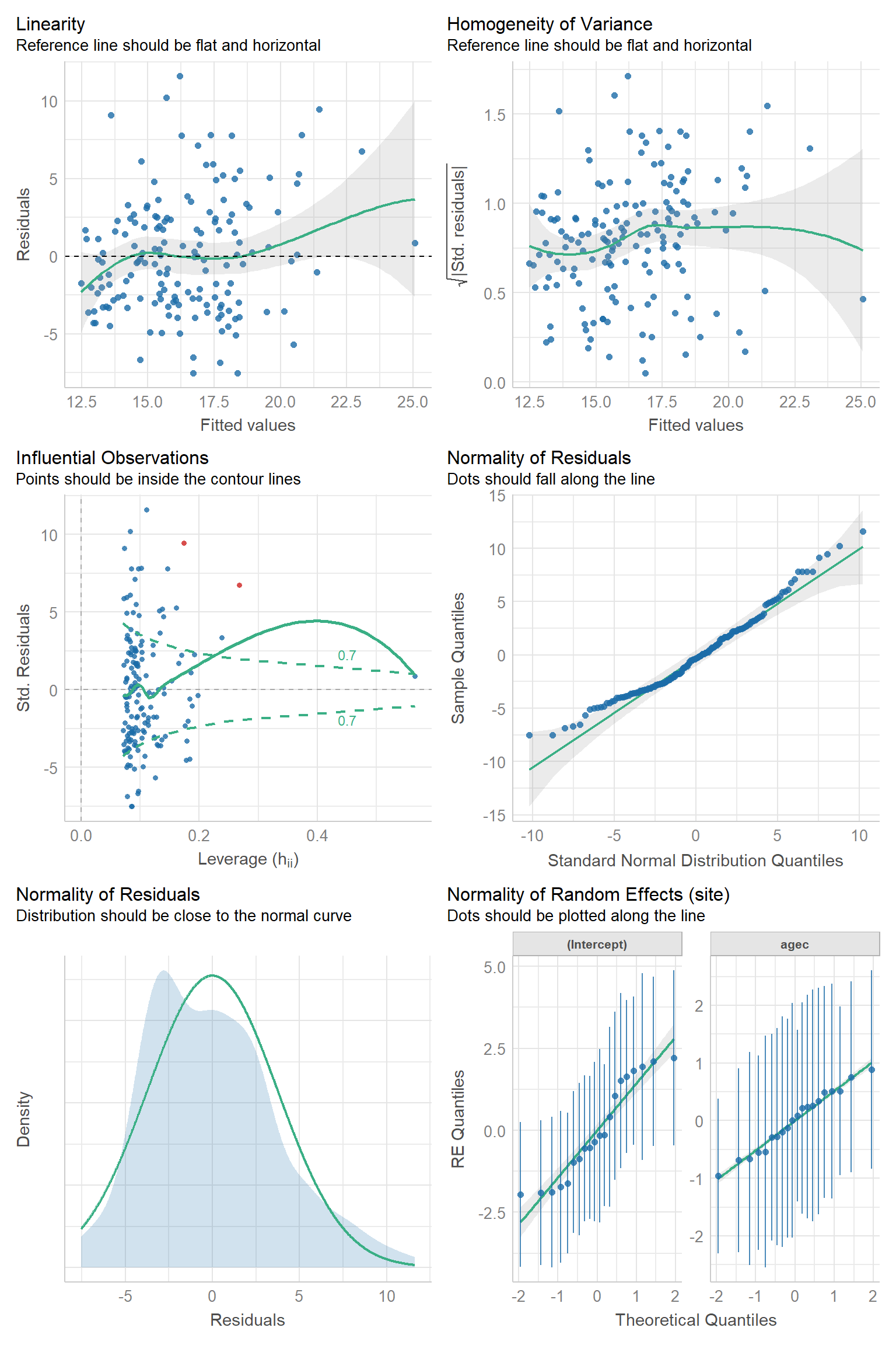
FIGURE 18.14: Residual diagnostic plots using the check_model function in the performance package (Lüdecke et al., 2021) for the random intercept and slope model fit to the pines data set.
Somewhat subjectively, I would conclude that there are no major issues with the assumptions of either model.
18.11 Model comparisons, hypothesis tests, and confidence intervals for fixed-effects and variance parameters
18.11.1 Estimation using restricted maximum likelihood (REML) or maximum likelihood (ML)
One topic we have avoided so far, but will come up when discussing hypothesis tests for fixed and random-effects parameters, is the difference between restricted maximum likelihood (REML) and maximum likelihood (ML) methods for estimating parameters. We briefly mentioned in Section 10.5 that the maximum likelihood estimator of \(\sigma^2\) for Normally distributed data is biased, and that we tend to use an unbiased estimator that divides by \(n-1\) instead of \(n\). It turns out that maximum-likelihood estimators of variance components in mixed-effect models are also biased. REML provides a similar correction by maximizing a modified form of the likelihood that depends on the fixed effects included in the model. Thus, REML is the default method used when fitting models using lmer. To estimate parameters using ML, we need to add the argument, method = "ML".
Why is this important? Comparisons of models with different fixed effects (e.g., using AIC or likelihood ratio tests) are not valid when using REML. Thus, a common recommendation is to use ML when comparing models (e.g., using likelihood ratio tests) that differ only in their fixed effects. However, it is generally accepted, and in fact recommended, to compare models that differ only in terms of their random effects using models fit using REML.
18.11.2 Hypothesis tests for fixed-effects parameters and degrees of freedom
To begin our journey to understand tests of fixed-effect parameters, we will explore output when fitting random intercept and random slope models using the lme function in the nlme package. The syntax will be a little different. Instead of specifying the random intercepts associated with each site using (1 | site), we will have a separate argument, random = ~ 1 | site. In both cases, we use 1 | site to tell R that we want the intercepts (i.e., the column of 1’s in the design matrix) to vary randomly by site.
## Linear mixed-effects model fit by REML
## Data: pines
## AIC BIC logLik
## 926.7807 939.0311 -459.3904
##
## Random effects:
## Formula: ~1 | site
## (Intercept) Residual
## StdDev: 2.053276 4.018271
##
## Fixed effects: dbh ~ agec
## Value Std.Error DF t-value p-value
## (Intercept) 16.47431 0.5608231 139 29.375226 0
## agec 2.43047 0.4100212 139 5.927671 0
## Correlation:
## (Intr)
## agec 0.012
##
## Standardized Within-Group Residuals:
## Min Q1 Med Q3 Max
## -1.92182870 -0.74556282 -0.05850252 0.60196036 2.88237383
##
## Number of Observations: 160
## Number of Groups: 20As with lmer, we end up with estimates of the mean intercept and slope in the population, \(\hat{\beta}_0 = 16.47\) and \(\hat{\beta_1} = 2.43\), respectively; we also see that lme provides estimates of the standard deviations of the site-level intercepts (\(\hat{\sigma}_{site} = 2.05\)) and within-site errors (\(\hat{\sigma}_{\epsilon} = 4.018\)). Unlike with the output from lmer, however, we also get a test statistic and p-value for null hypothesis tests that \(\beta_0 = 0\) and \(\beta_1 = 0\) based on a t-distribution with \(df = 139\). This test is only approximate and there are better ways to conduct hypothesis tests (e.g., using simulation based approaches as discussed in Section 18.11.5). Thus, the developers of the lme4 package decided it would be best not to provide p-values when summarizing the output of a model fit using lmer. Nonetheless, the default method that lme uses to determine degrees of freedom is instructive, particularly if we fit models that include level-1 and level-2 covariates (i.e., variables that do and do not vary within each site):
## Linear mixed-effects model fit by REML
## Data: pines
## AIC BIC logLik
## 920.0064 941.3103 -453.0032
##
## Random effects:
## Formula: ~1 | site
## (Intercept) Residual
## StdDev: 1.994415 3.99883
##
## Fixed effects: dbh ~ agec + Aspect
## Value Std.Error DF t-value p-value
## (Intercept) 18.337679 1.1513720 139 15.926807 0.0000
## agec 2.679396 0.4435988 139 6.040134 0.0000
## AspectNorth -1.362490 1.6508010 16 -0.825351 0.4213
## AspectSouth -2.681490 1.5738823 16 -1.703742 0.1078
## AspectWest -3.376375 1.6551813 16 -2.039883 0.0582
## Correlation:
## (Intr) agec AspctN AspctS
## agec 0.310
## AspectNorth -0.732 -0.329
## AspectSouth -0.711 -0.160 0.514
## AspectWest -0.741 -0.363 0.558 0.518
##
## Standardized Within-Group Residuals:
## Min Q1 Med Q3 Max
## -1.85312474 -0.71672171 -0.07700017 0.55987900 2.77709336
##
## Number of Observations: 160
## Number of Groups: 20In this case, we see that the p-values associated with the coefficients for Apsect are based on a t-distribution with only 16 degrees of freedom. The exact formulas used to calculate these default degrees of freedom (provided below) are not important (again, there are now better ways to conduct these tests) – what is important is that we have much less information about predictors that do not vary within a cluster than we do about predictors that do vary within a cluster. For level-1 predictors, lme calculates the within-subjects degrees of freedom as the number of observations minus the number of clusters minus the number of level-1 predictors in the model. For level-2 predictors, lme calculates degrees of freedom using the number of clusters minus the number of level-2 predictors the model - 1 for the intercept.
[1] 139[1] 16Again, these formula are not that important. What is important is that lme attempts to account for the data structure when carrying out statistical tests, recognizing that the site is the correct unit of replication for tests involving Aspect. The default degrees of freedom calculated by lme are essentially correct for balanced data (where you have equal numbers of observations within each cluster), assuming the model assumptions hold. For unbalanced data, the tests (and degrees-of-freedom) are only approximate.
18.11.3 Alternative methods for testing hypotheses about fixed effects
Various other methods for approximating degrees of freedom have been suggested, and these methods are implemented in the lmerTest and pbkrtest packages (Halekoh & Højsgaard, 2014; Kuznetsova, Brockhoff, & Christensen, 2017). If the lmerTest function has been loaded, you will automatically see tests using a t-distribution with Satterthwaite’s degrees of freedom, a method you may have seen when learning about a t-test for a difference in means with unequal variances (Giesbrecht & Burns, 1985; Hrong-Tai Fai & Cornelius, 1996).
library(lmerTest)
lmer.ri <- lmer(dbh ~ agec + (1 | site), data = pines) #lme4 package
summary(lmer.ri)
## Linear mixed model fit by REML. t-tests use Satterthwaite's method [
## lmerModLmerTest]
## Formula: dbh ~ agec + (1 | site)
## Data: pines
##
## REML criterion at convergence: 918.8
##
## Scaled residuals:
## Min 1Q Median 3Q Max
## -1.9218 -0.7456 -0.0585 0.6020 2.8824
##
## Random effects:
## Groups Name Variance Std.Dev.
## site (Intercept) 4.216 2.053
## Residual 16.147 4.018
## Number of obs: 160, groups: site, 20
##
## Fixed effects:
## Estimate Std. Error df t value Pr(>|t|)
## (Intercept) 16.4743 0.5608 13.8574 29.375 7.02e-14 ***
## agec 2.4305 0.4100 108.5317 5.928 3.70e-08 ***
## ---
## Signif. codes: 0 '***' 0.001 '**' 0.01 '*' 0.05 '.' 0.1 ' ' 1
##
## Correlation of Fixed Effects:
## (Intr)
## agec 0.012We see that the degrees of freedom are smaller (and p-values are larger) than those reported by default by lme, particularly for the intercept. Another popular method for calculating degrees of freedom is the method proposed by Kenward and Rodger (Kenward & Roger, 1997). This approximation can be used to compare two nested models using the KRmodcomp function in the pbkrtest package (Halekoh & Højsgaard, 2014). Alternatively, tests using Kenward-Rodger degrees of freedom can be calculated by adding ddf = "Kenward-Roger" when using the summary function with a model fitted using lmer:
## Linear mixed model fit by REML. t-tests use Kenward-Roger's method [
## lmerModLmerTest]
## Formula: dbh ~ agec + (1 | site)
##    Data: pines
##
## REML criterion at convergence: 918.8
##
## Scaled residuals:
##     Min      1Q  Median      3Q     Max
## -1.9218 -0.7456 -0.0585  0.6020  2.8824
##
## Random effects:
##  Groups   Name        Variance Std.Dev.
##  site     (Intercept)  4.216   2.053
##  Residual             16.147   4.018
## Number of obs: 160, groups:  site, 20
##
## Fixed effects:
##             Estimate Std. Error       df t value Pr(>|t|)
## (Intercept)  16.4743     0.5611  18.3642  29.358  < 2e-16 ***
## agec          2.4305     0.4208 118.5132   5.776 6.29e-08 ***
## ---
## Signif. codes:  0 '***' 0.001 '**' 0.01 '*' 0.05 '.' 0.1 ' ' 1
##
## Correlation of Fixed Effects:
##      (Intr)
## agec 0.012
These alternative degrees of freedom have also been implemented in conjunction with the anova function (lmerTest also switches the default from sequential, added-in-order tests to backwards elimination tests - see Section 3.9). For example, we now have non-integer degrees of freedom if we consider testing for an effect of Aspect in a model that also contains age:
## Type III Analysis of Variance Table with Satterthwaite's method
##        Sum Sq Mean Sq NumDF   DenDF F value    Pr(>F)
## agec   583.39  583.39     1 144.061 36.4832 1.249e-08 ***
## Aspect  82.44   27.48     3  13.972  1.7186     0.209
## ---
## Signif. codes:  0 '***' 0.001 '**' 0.01 '*' 0.05 '.' 0.1 ' ' 1
Further, the order of entry no longer matters:
## Type III Analysis of Variance Table with Satterthwaite's method
##        Sum Sq Mean Sq NumDF   DenDF F value    Pr(>F)
## Aspect  82.44   27.48     3  13.972  1.7186     0.209
## agec   583.39  583.39     1 144.061 36.4832 1.249e-08 ***
## ---
## Signif. codes:  0 '***' 0.001 '**' 0.01 '*' 0.05 '.' 0.1 ' ' 1
Luke (2017) compared type I error rates for likelihood ratio tests and tests using Kenward-Roger or Satterthwaite approximations and found the latter two approaches performed well.
Lastly, to reinforce the need to consider random slopes for predictors that vary within a cluster, let’s compare the degrees of freedom and the p-values for the fixed effects parameters with and without the random slope:
## Type III Analysis of Variance Table with Satterthwaite's method
##        Sum Sq Mean Sq NumDF   DenDF F value    Pr(>F)
## agec   583.39  583.39     1 144.061 36.4832 1.249e-08 ***
## Aspect  82.44   27.48     3  13.972  1.7186     0.209
## ---
## Signif. codes:  0 '***' 0.001 '**' 0.01 '*' 0.05 '.' 0.1 ' ' 1
lmer.rc2 <- lmer(dbh ~ agec + Aspect + (1 + agec | site), data = pines) #lme4 package
anova(lmer.rc2)## Type III Analysis of Variance Table with Satterthwaite's method
## Sum Sq Mean Sq NumDF DenDF F value Pr(>F)
## agec 488.34 488.34 1 15.462 31.5029 4.418e-05 ***
## Aspect 74.26 24.75 3 13.777 1.5968 0.2355
## ---
## Signif. codes: 0 '***' 0.001 '**' 0.01 '*' 0.05 '.' 0.1 ' ' 1We see that including the random slope does little to change the degrees of freedom (or p-value) for the test associated with Apsect, but it has a big effect on the test for age, resulting in a much more conservative test with larger p-value!
18.11.4 Confidence intervals for fixed effects and variance parameters
We can use the confint function along with models fit using lmer to generate confidence intervals using the profile-likelihood method (the default; see Section 10.9), using bootstrapping (by specifying method = "boot"), or using a large-sample approximation based on assuming the sampling distribution is Normal (method = "Wald"); the latter approach is only available for fixed-effects coefficients since the sampling distribution of variance parameters tends to be right-skewed and thus, far from Normal. The profile-likelihood and bootstrap confidence intervals are to be preferred, but they can be computationally intensive to compute. By contrast, the Wald method is simple and fast; these intervals are calculated simply as \(\hat{\beta} \pm 1.96 SE(\hat{\beta})\) When calculating profile-likelihood and bootstrap confidence intervals, you will often see warnings related to computational issues (e.g., non-convergence associated with 1 or more bootstrapped data sets). In those cases, it is useful to also compute Wald intervals to see how they compare.
We compare these three approaches for the random intercepts and slopes model, below. We have suppressed warnings and messages, but if you run the code on your own, you will be able to see them.
conf.pl <- confint(lmer.rc, method = "profile")
conf.boot <- confint(lmer.rc, method = "boot")
conf.norm <- confint(lmer.rc, method = "Wald")
confs <- data.frame(rbind(conf.pl, conf.boot, conf.norm))
names(confs) <- c("LCL", "UCL")
confs$term <- as.factor(rep(c("sigma[b0]","sigma[b1]", "cov(b0, b1)",
                              "sigma[epsilon]", "beta[0]", "beta[1]"), 3))
confs$method <- rep(c("Profile likelihood", "conf.boot", "conf.norm"),
                    each = nrow(conf.pl))

# Note the estimates are given in a slightly different order than the confidence intervals
confs$estimate <- rep(c(as.data.frame(VarCorr(lmer.rc))$sdcor[c(1,3, 2, 4)],
                        fixef(lmer.rc)), 3)
ggplot(confs, aes(method, estimate)) + geom_point() +
  geom_errorbar(aes(ymin=LCL, ymax=UCL), width=0.2) +
  facet_wrap(~term, scales="free")+
  theme(axis.text.x = element_text(angle = 45, hjust = 1))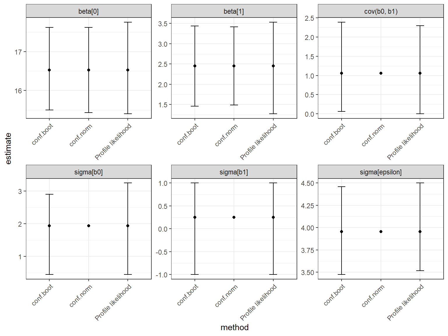
FIGURE 18.15: Comparison of different methods (profile likelihood, bootstrap, Wald) for computing confidence intervals for fixed-effects and variance parameters in mixed-effects models.
Examining Figure 18.15, we see that for this particular data set, the three intervals are all fairly similar.
18.11.5 Simulation-based testing: Comparing models with different random-effect structures
As mentioned in the previous section, the sampling distributions for variance parameters tend to be right skewed. Therefore, tests based on a Normal or t-distribution are not likely to be appropriate. We could consider using a likelihood ratio test to compare nested models (e.g., models with and without a random effects), thereby testing whether one or more variance parameters are 0. For example, we could compare our random intercept model with a random intercept and slope model to test:
\[H_0: \sigma^2_{b1} = 0 \text{ versus } H_A: \sigma^2_{b1} \ne 0\]
However, this test will be conservative since, under the null hypothesis, \(\sigma^2_{b1}\) is “on the boundary” of the parameter space – i.e., \(H_0: \sigma^2_{b_1} = 0\), sets the parameter \(\sigma^2_{b_1}\) to the boundary of what is possible for this parameter (variance parameters cannot go negative). When this is the case, p-values and comparisons using AIC need adjustment (see e.g., Self & Liang, 1987). Pinheiro & Bates (2006) note that the p-value for a likelihood ratio test involving a single variance parameter will be approximately twice as large as it should be. They suggest that the sampling distribution associated with the likelihood-ratio \(\chi^2\) statistic comparing models that differ by 1 parameter (set to the boundary of its parameter space) can be approximated as a 50:50 mixture of a \(\chi^2_1\) and a \(\chi^2_2\) distribution. In this case, we could calculate an approximate p-value using: 0.5 + 0.5qchisq(LR, 1), where LR is the likelihood-ratio statistic calculated by comparing our two models.
Alternatively, we can calculate a p-value using a simulation-based test. Let’s consider comparing the random intercept and random intercept and slope models. Our null hypothesis would be that the simpler model containing only random intercepts is appropriate for the data. The alternative hypothesis is that the more complicated random intercepts and slope model fits the data better. Recall that with any null hypothesis test, we need a test statistic and a distribution of that test statistic when the null hypothesis is true. We can use the likelihood-ratio statistic as our test statistic, but rather than rely on an assumed \(\chi^2_1\) distribution, we can generate the distribution of the test statistic when the null hypothesis is true using simulations from the null model (Crainiceanu & Ruppert, 2004). This will require that we:
- Simulate data under the null (i.e., smaller) model; a parametric bootstrap can be used here to simulate data from the fitted random-intercept model.
- Fit the two nested models (random intercept only model, random intercept and slope model) to the simulated data
- Calculate the likelihood ratio statistic comparing the fitted models to the simulated data.
Steps 1-3 will be repeated several times to generate the null distribution of the likelihood ratio statistic. We can then calculate a p-value for the test by comparing the observed likelihood ratio statistic using the actual data to the above null distribution.
The RLRsim (Scheipl, Greven, & Kuechenhoff, 2008) and pbkrtest (Halekoh & Højsgaard, 2014) packages provide functions for conducting simulation-based tests. Below, we demonstrate the PBmodcomp function in the pbkrtest package for conducting the hypothesis test.
## Bootstrap test; time: 13.53 sec; samples: 500; extremes: 165;
## Requested samples: 500 Used samples: 497 Extremes: 165
## large : dbh ~ agec + (1 + agec | site)
## dbh ~ agec + (1 | site)
##            stat      df    ddf p.value
## LRT      1.0803 2.00000         0.5827
## PBtest   1.0803                 0.3333
## Gamma    1.0803                 0.3413
## Bartlett 1.8541 2.00000         0.3957
## F        0.5401 2.00000 14.098  0.5943
PBmodcomp provides several tests using different test statistics, including the likelihood ratio test statistic (given by the LRT line). The p-values for all of these tests are large, suggesting there is not much evidence to support the more complicated model that also includes random slopes. Nonetheless, it is often best to choose the structure of the random effects to match the experimental design or structure of your data rather than base this choice on a null hypothesis test (Arnqvist, 2020). We will further discuss methods for choosing an appropriate model in Section 18.12.
18.11.6 Comparisons using AIC
It is also tempting to use AIC to compare models – e.g., the random intercept model and the model that also includes a random slope:
        df      AIC
lmer.ri  4 926.7807
lmer.rc  6 929.3578
The use of AIC for mixed models is not straightforward. Consider counting the number of parameters in the random-intercept model. We might choose to count the 2 fixed effects parameters, the variance of the random intercepts, and the variance of the within-site errors, so 4 parameters. This could be appropriate if we are mainly interested in making inference to the population of sites. On the other hand, we might be interested in estimating site-specific response patterns. In that case, our parameters might be closer to 3 + the number of sites -1. These issues, related to the “level of focus” are discussed in Vaida & Blanchard (2005) and Greven & Kneib (2010). In addition, like likelihood ratio tests, the comparison between the random intercept and random intercept and slope model involves setting a variance parameter to a value “on the boundary” of the parameter space (as discussed in Section 18.11.5). Using AIC calculated using the first approach tends to be conservative, leading to simpler models (Greven & Kneib, 2010). For more discussion of these topics, I highly recommend visiting Ben Bolker’s GLMM FAQ page.
18.12 Modeling strategies revisited
We saw in Section 8 how challenging it can be to select an appropriate model when allowed freedom to choose among several predictors. These challenges are even more pronounced when fitting mixed-effects models, and again, we will find that there are different viewpoints on how best to go about choosing an appropriate model.
18.12.1 Fixed versus random effects
As a first step, analysts must choose whether to model the effect of categorical variables (and their interactions with other continuous variables) as fixed or random effects. Guidance here is often based on:
how many levels (i.e., clusters or groups) are associated with the categorical variable. If there are few clusters (e.g., < 5 or 10), then it may be best to model using fixed effects since it can be really difficult to estimate variance parameters with so few replicates. On the other hand, it may be OK to include a factor as a random effect if the main reason to do so is to account for a feature of the data (e.g., an experimental design that results in hierarchical data). Although the variance component associated with the factor may be imprecisely estimated, it may still control the type I error. In fact, either approach (including a factor as random or fixed) is likely going to control the type I error rate and is preferable to ignoring clustering in the data and treating the observations as though they were independent (see e.g., Oberpriller, Souza Leite, & Pichler, 2021).
whether the focus is on the specific clusters (e.g., sites) that were observed or one wants to make inference to a larger population. In the latter case, mixed-effects models are preferable since they estimate coefficients describing mean effects and their variance across different clusters.
Assuming one chooses to model using random effects, then one is faced with questions about the structure of the random effects as well as which variables to include in the fixed effects part of the model.
18.12.2 Maximal model
As we mentioned previously, too often ecologists default to fitting random-intercept models. Doing so often results in models that fail to control type I error rates in the face of pseudoreplication (Schielzeth & Forstmeier, 2009). At the other extreme, is the recommendation to fit a maximal model with as many random coefficients as possible (i.e., for all predictors that vary within a cluster) (Barr, Levy, Scheepers, & Tily, 2013). Although this sounds appealing from a type I error perspective, in reality, it is often difficult to fit a model with multiple random coefficients. When faced with convergence problems, this often leads to a haphazard model-selection process in an attempt to find a simpler model that converges.
One simple thing you can do to improve the chances that the optimizer used to estimate parameters converges is to scale and center your continuous variables. We did this with age when fitting mixed models to the pines data. We would have encountered issues with fitting the random slope model if we had not done this (see below):
## Warning in checkConv(attr(opt, "derivs"), opt$par, ctrl = control$checkConv, :
## Model failed to converge with max|grad| = 1.16634 (tol = 0.002, component 1)
## Warning in checkConv(attr(opt, "derivs"), opt$par, ctrl = control$checkConv, : Model is nearly unidentifiable: very large eigenvalue
## - Rescale variables?## Linear mixed model fit by REML ['lmerModLmerTest']
## Formula: dbh ~ age + (age | site)
## Data: pines
## REML criterion at convergence: 925.3739
## Random effects:
## Groups Name Std.Dev. Corr
## site (Intercept) 2.67944
## age 0.01718 -0.73
## Residual 3.96886
## Number of obs: 160, groups: site, 20
## Fixed Effects:
## (Intercept) age
## 9.45435 0.04629
## optimizer (nloptwrap) convergence code: 0 (OK) ; 0 optimizer warnings; 2 lme4 warnings18.12.3 Top-down model-selection
Largely following Diggle, Liang, & Zeger (1994), Zuur et al. (2009) suggests a “top-down” strategy for choosing an appropriate model. They note that tests for fixed effects will be wrong if the structure of the random effects is too simple. In addition, they note that random effects can soak up variation that could be due to the omission of important fixed effects. Thus, they suggest an iterative approach involving the following 5 steps:
- Start with a “full model” that contains as many covariates of interest as possible.
- Compare different random effects structures (e.g., models with random intercepts versus random slopes) using AIC or likelihood-ratio tests (see Section 18.11.5). During this step, they suggest using
method = "REML"since it will give better estimates of variance parameters.
- Once an appropriate random-effects structure is chosen, they then compare models with different fixed effects, again using AIC and likelihood-ratio tests but with
method = "ML". During this stage, they keep the random effects structure constant based on the results from step 2. - Once the fixed effects are chosen, they recommend refitting the final model but with
method = "REML". At this point, they also recommend evaluating the assumptions of the model (see Section 18.10)
18.12.4 A multi-level bottom-up approach to model selection
Others, including Jack Weiss and Singer, Willett, Willett, & others (2003) recommend a bottom up approach that begins by fitting the following models (Figure 18.16):
- Pooled model (assuming independence), include level-1 predictors [predictors that vary within clusters]
lm(y ~ x1) - Unconditional means model or variance components model (no predictors, just random intercepts)
lmer(y ~ 1 +(1 | site)) - Random intercepts (with level 1 predictors )
lmer(y ~ x1 + (1 | site)) - Random intercepts and slopes (with level 1 predictors)
lmer(y ~ x1 + (1 + x1 | site))
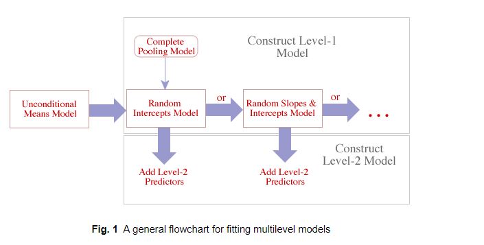
FIGURE 18.16: Multi-level modeling strategy (Figure from Jack Weiss’s web pages).
After picking the best of these models, they then suggest adding level-2 predictors (predictors that are constant within clusters).
Let’s apply this approach to our pines data. Here, we use AIC, not withstanding the concerns raised earlier (see Section 18.11.6).
pooled.model <- lm(dbh ~ agec, data = pines)
uncond.means.model <- lmer(dbh ~ 1 + (1 | site), data = pines)
randint.model <- lmer(dbh ~ 1 + agec + (1 | site), data = pines)
randcoef.model <- lmer(dbh ~ 1 + agec + (agec | site), data = pines)
AIC(pooled.model, uncond.means.model, randint.model, randcoef.model)
## df AIC
## pooled.model 3 932.4945
## uncond.means.model 3 953.2307
## randint.model 4 926.7807
## randcoef.model 6 929.3578This comparison suggests that the random intercept model has the lowest AIC. We also failed to find evidence for the random intercept and slope model using the simulation-based likelihood ratio test in Section 18.11.5. Thus, we might consider adding level-2 covariates (e.g., Apect) to the random intercept model.
We can then compare this model to the model without Aspect using either hypothesis tests or AIC.
## Type III Analysis of Variance Table with Satterthwaite's method
##        Sum Sq Mean Sq NumDF   DenDF F value    Pr(>F)
## agec   583.39  583.39     1 144.061 36.4832 1.249e-08 ***
## Aspect  82.44   27.48     3  13.972  1.7186     0.209
## ---
## Signif. codes: 0 '***' 0.001 '**' 0.01 '*' 0.05 '.' 0.1 ' ' 1## df AIC
## lmer.ri 4 926.7807
## lmer.ri2 7 920.0064The evidence for the importance of Aspect is fairly week, despite resulting in a model with lower AIC.
18.13 Induced corrlation, marginal model, generalized least squares
As we noted earlier, many ecologists add random intercepts mainly as a way to avoid issues related to “pseudeoreplication” or non-independence (even though random slopes may be needed to guard against inflated type I error rates; Schielzeth & Forstmeier, 2009). In this section, we briefly highlight how adding random effects induces correlation among observations that share the same values of the random effect. We will also show an equivalence between the random-intercept model and a marginal model with compound symmetry that can be fit using the gls function in the nlme package.
Recall from Section 9.7, that the variance of two random variables, \(X\) and \(Y\) is given by:
\(var(X + Y) = var(X)+ var(Y) + 2cov(X, Y)\)
In addition, the covariance of \(X\) and \(Y\) is given by: \(cov(X,Y) = E[XY] - E[X]E[Y]\). If we consider the random intercepts model, we have 2 random terms, \(b_{0i}\) and \(\epsilon_{ij}\):
\[\begin{equation} dbh_{ij} = \beta_0 + b_{0i}+ \beta_1age_{ij} + \epsilon_{ij} \end{equation}\]
Thus, it is easy to derive the following:
\(var(dbh_{ij}) = var(b_{0i}+\epsilon_{ij}) = var(b_{0i}) +var(\epsilon_{ij}) = \sigma_{b_0}^2 + \sigma_{\epsilon}^2\)
\(cov(dbh_{ij}, dbh_{ij^\prime}) = \sigma^2_{b_0}\) (for any 2 observations collected at the same site since they will share \(b_{0i}\)); in addition, the correlation between any two observations from the same site = \(cor(dbh_{ij}, dbh_{ij^\prime})\) = \(\frac{\sigma_{b_0}^2}{\sigma_{b_0}^2+\sigma^2_{\epsilon}}\).
\(cov(dbh_{ij}, dbh_{i^\prime j}) = 0\) (for any 2 observations taken from 2 different sites since they will not share \(b_{0i}\) or \(\epsilon_{ij}\))
We can also derive the marginal distribution of our response variable by averaging over the distribution of the random effects (see Section 9.8 for a discussion of conditional versus marginal distributions).
Let’s start by writing down equations for the random intercept model in terms of the conditional distribution of \(Y | b\) and the distribution of \(b\) as in Section 18.7.
\[\begin{gather} dbh_{ij} | b_{0i} \sim N(\mu_i, \sigma^2_{\epsilon}) \\ \mu_{ij} = (\beta_0 +b_{0i}) + \beta_1age_{ij} \tag{18.9} \\ b_{0i} \sim N(0, \sigma^2_{b_0}) \end{gather}\]
If we average over (or integrate out) the random effects, \(b_{0i}\), we get the marginal Distribution of \(Y\). This distribution can be derived analytically in the case of linear mixed-effects models, and allows us to write down a likelihood for the data that does not involve the random effects. The marginal likelihood is what R uses when it estimates \(\beta_0\), \(\beta_1\), and the variance parameters, \(\sigma^2_{b0}\) and \(\sigma^2_{\epsilon}\). For the random-intercept model, the marginal distribution for the vector of observations from site \(i\), \(Y_i\), is given by:
\[\begin{gather} Y_{i}\sim N(X_{i}\beta, V_i) \\ V_i = \begin{bmatrix} \sigma^2_{\epsilon} + \sigma^2_{b_0} & \sigma^2_{b_0} & \cdots & \sigma^2_{b_0} \\ \sigma^2_{b_0} & \sigma^2_{\epsilon} + \sigma^2_{b_0} & \sigma^2_{b_0} & \sigma^2_{b_0} \\ \vdots & \ddots & \ddots & \vdots \\ \sigma^2_{b_0} & \cdots & \sigma^2_{b_0} & \sigma^2_{\epsilon} + \sigma^2_{b_0} \end{bmatrix} \tag{18.10} \end{gather}\]
Here, \(V_i\) gives the variance covariance matrix for the observations from site \(i\) and has dimension \(n_i \times n_i\). The diagonal elements hold the variances and the off-diagonal elements hold the covariances that we derived above. If we consider all of the data, not just the observations from site \(i\), then we have:
\[\begin{gather} Y \sim N(X\beta, \Sigma) \\ \Sigma = \begin{bmatrix} V_1 & 0 & 0 & 0 \\ 0 & V_2 & 0 & 0 \\ \vdots & \ddots & \ddots & \vdots \\ 0 & \cdots & 0 & V_{40} \end{bmatrix} \end{gather}\]
Here, \(\Sigma\) is the variance/covariance matrix for all of the observations. This matrix is what is referred to as block diagonal. The 0’s represent covariances for observations from different sites – these are 0, since we assume observations from different sites are independent. The \(V_i\) contain the variance/covariances for cluster \(i\) (eq. (18.10)).
Thus, the random intercept model is equivalent to assuming that all observations from the same site (or cluster) are equally correlated, and that observations from different sites (or clusters) are independent. This particular form of correlation is referred to as compound symmetry. Rather than fitting a random intercepts model, we could have posited this model as one that would be reasonable for our data a priori. Specifically, we could consider the vector of response data and directly model their multivariate mean and variance covariance matrix. The gls function in the nlme package will let us do just that.
gls.fit<-gls(dbh ~ agec, method="REML",
             correlation=corCompSymm(form= ~ 1 | site),
            data=pines)
summary(gls.fit)
Generalized least squares fit by REML
Model: dbh ~ agec
Data: pines
AIC BIC logLik
926.7807 939.0311 -459.3904
Correlation Structure: Compound symmetry
Formula: ~1 | site
Parameter estimate(s):
Rho
0.2070437
Coefficients:
Value Std.Error t-value p-value
(Intercept) 16.474305 0.5608219 29.375289 0
agec 2.430468 0.4100210 5.927666 0
Correlation:
(Intr)
agec 0.012
Standardized residuals:
Min Q1 Med Q3 Max
-2.1264342 -0.7593302 -0.2326614 0.4739741 3.0916412
Residual standard error: 4.512474
Degrees of freedom: 160 total; 158 residual(Intercept) agec
16.474305 2.430471 Note that we get the exact same fixed effects coefficients as when fitting the random intercept model. In addition, the estimate of the intraclass correlation that is returned by gls = 0.207 is equivalent to \(\frac{\hat{\sigma}^2_{b_0}}{\hat{\sigma}^2_{\epsilon} + \hat{\sigma}^2_{b_0}}\) from the random intercept model, and the residual standard error from the gls model is equal to \(\sqrt{\hat{\sigma}^2_{\epsilon} + \hat{\sigma}^2_{b_0}}\)
# Extract variance parameters from the random intercept model
variancepars<-as.data.frame(VarCorr(lmer.ri))

# rho calculated from random intercept model
variancepars[1,4]/(variancepars[1,4]+variancepars[2,4])
## [1] 0.207045## [1] 4.512476As was mentioned in Section 9.11.1, the Normal distribution is unique in that it has separate parameters for the mean and for the variance (and covariance terms). There is no multivariate analogue of other commonly used statistical models (e.g., the Binomial or Poisson distribution) that allow one to directly model the mean and variance/covariance. We will follow up on this point in Section 19.
18.14 Random effects specified using multiple grouping variables
You may find that you have multiple categorical variables that could be considered as grouping variables for structuring random effects. For example, if you follow multiple individuals over several years, you might consider adding a random intercept for each individual to model correlation among observations from the same individual or a random intercept for each year to allow for correlation among observations in the same year. In this section, we will also see that it is possible to include random intercepts (and, potentially, random slopes) using more than one grouping variable (e.g., individual and year).
We will consider data from Dickie et al. (2022), who explored associations between wolf home-range size and measures of primary productivity and the extent of linear features (e.g., roads) within individuals’ home ranges. Data from this study are included in the Data4Ecologists package in the HRData data set and can be accessed using:
In addition to having repeated observations on individuals over time (home ranges were estimated seasonally and annually), more than one wolf was observed from some wolf packs (Figure 18.17). Thus, we might consider including AnimalID, PackID, and Year as grouping variables for random effects (i.e., random intercepts or random coefficients).
HRsummary <- HRData %>% group_by(PackID, Year) %>%
  count()
ggplot(HRsummary, aes(Year, PackID, size = n)) + geom_point() +
  ylab("Pack ID")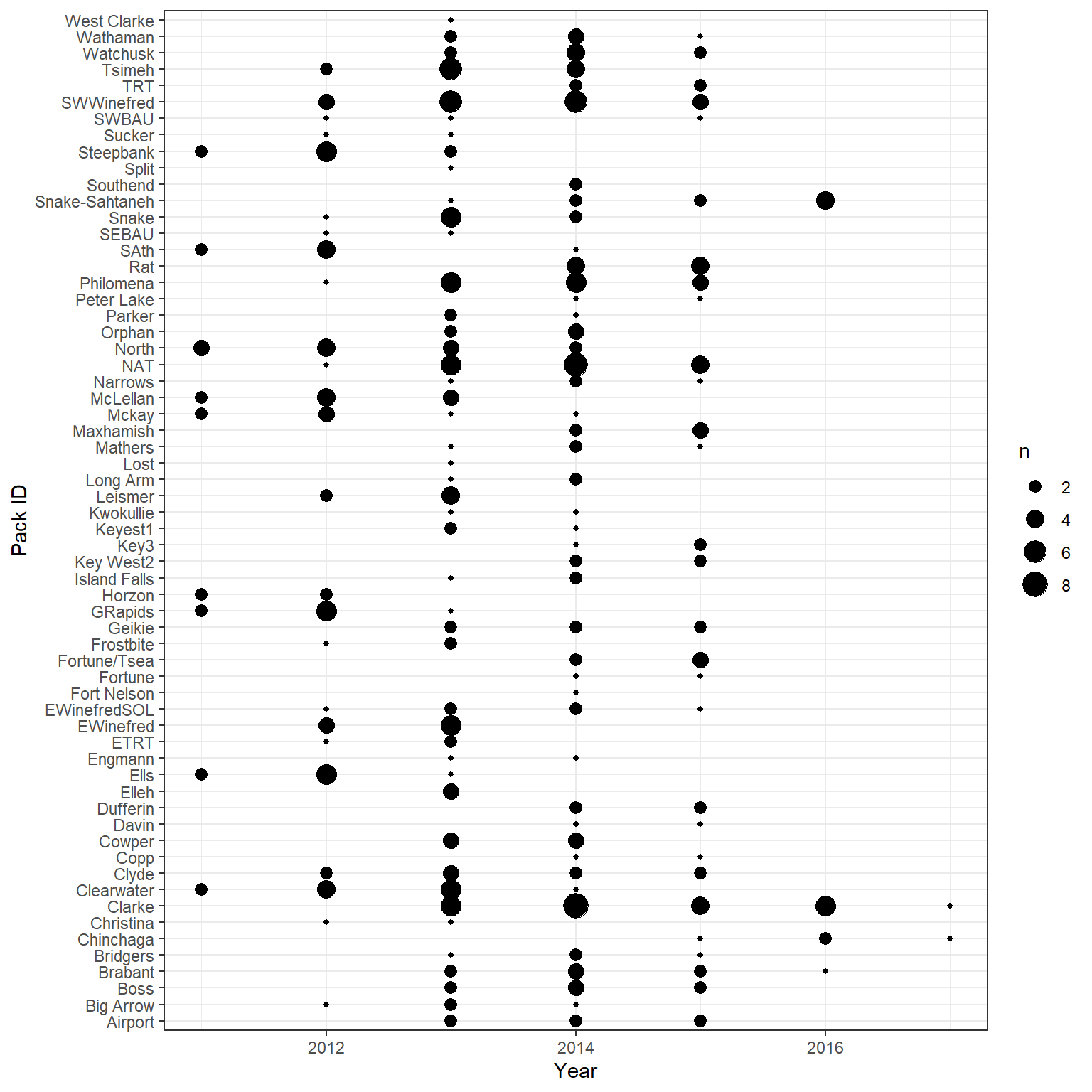
FIGURE 18.17: Number of observations of estimated home-range size for each of several wolf packs in the HRData data set from Dickie et al. (2022).
Dickie et al. (2022) considered models with the following fixed effects:
Season= snow (Nov-April) or snow-free (May-October)StudyArea(SAin their original data set) = BC for northeastern British Columbia, WHEC for northern Alberta, RICC for northeastern Alberta, and SK for SaskatchewanDiffDTScaled= the number of days of monitoring data associated with the home-range estimate, scaled between 0 and 1EVIScaled= a scaled measure of primary productivity within the estimated home ranges (assumed to influence the abundance of wolf prey)LFD= density of linear features (LFD) within the estimated home ranges.
They also considered an interaction between EVIScaled and LFD to determine if the effect of linear features depended on resource density. Dickie et al. (2022) compared three different models, each with a different random-effects specification. I find their choice of models a bit strange (see Section 18.14.1). Instead, let’s begin by considering the following model:
model1 <- lmer(log(HRsize) ~ Season + StudyArea + DiffDTScaled + LFD*EVIScaled +
                     (1 | AnimalId) + (1 | Year),  REML=TRUE, data = HRData)
summary(model1)
## Linear mixed model fit by REML. t-tests use Satterthwaite's method [
## lmerModLmerTest]
## Formula: log(HRsize) ~ Season + StudyArea + DiffDTScaled + LFD * EVIScaled +
## (1 | AnimalId) + (1 | Year)
## Data: HRData
##
## REML criterion at convergence: 718.4
##
## Scaled residuals:
## Min 1Q Median 3Q Max
## -3.1974 -0.5314 -0.0044 0.5087 2.6537
##
## Random effects:
## Groups Name Variance Std.Dev.
## AnimalId (Intercept) 0.20867 0.4568
## Year (Intercept) 0.03643 0.1909
## Residual 0.28067 0.5298
## Number of obs: 359, groups: AnimalId, 142; Year, 7
##
## Fixed effects:
## Estimate Std. Error df t value Pr(>|t|)
## (Intercept) 9.50774 0.41954 232.87651 22.662 < 2e-16 ***
## SeasonSnowFree -0.48662 0.07464 242.09915 -6.519 4.07e-10 ***
## StudyAreaRICC -0.94537 0.15550 127.37452 -6.079 1.30e-08 ***
## StudyAreaSK -1.27522 0.27456 165.51587 -4.645 6.91e-06 ***
## StudyAreaWHEC -1.30407 0.18430 151.99775 -7.076 5.10e-11 ***
## DiffDTScaled 0.40872 0.10629 293.98415 3.845 0.000148 ***
## LFD -4.87658 1.80615 328.18140 -2.700 0.007294 **
## EVIScaled -2.47882 0.57135 269.65609 -4.339 2.03e-05 ***
## LFD:EVIScaled 5.09616 2.83954 334.21395 1.795 0.073603 .
## ---
## Signif. codes: 0 '***' 0.001 '**' 0.01 '*' 0.05 '.' 0.1 ' ' 1
##
## Correlation of Fixed Effects:
## (Intr) SsnSnF SARICC StdASK SAWHEC DffDTS LFD EVIScl
## SeasonSnwFr -0.015
## StudyArRICC -0.352 0.004
## StudyAreaSK -0.842 0.036 0.542
## StudyArWHEC -0.388 -0.050 0.647 0.542
## DiffDTScald -0.068 -0.507 -0.042 -0.006 -0.051
## LFD -0.698 0.008 0.102 0.525 0.098 -0.017
## EVIScaled -0.849 -0.005 -0.005 0.585 0.036 -0.002 0.713
## LFD:EVIScld 0.601 0.002 0.025 -0.370 0.040 0.005 -0.963 -0.729Writing down a set of equations for the model is challenging due to the incorporation of multiple categorical variables, including our grouping variables for the random effects (Year and AnimalId) and other categorical predictors modeled using fixed effects (Season, StudyArea). We will use indicator variables as in Section 3 to represent fixed effects predictors associated with the categorical variables Season and StudyArea. Let \(Y_{ij}\) be the home-range size for \(j^{th}\) observation associated with individual \(i\). Further, let \(b_{i}\) and \(\gamma_{k(ij)}\) represent random intercepts associated with individual \(i\) and year \(k\) (where the \(k(ij)\) subscript indicates the \(j^{th}\) observation of individual \(i\) is from year \(k\)). One option for describing the model is as follows:
\[\begin{gather} Y_{ij} | b_{i}, \gamma_{k(ij)} \sim N(\mu_{ij}, \sigma^2_{\epsilon}) \\ \mu_{ij} = \beta_0 + b_{i} + \gamma_{k(ij)} + \beta_1I(Season = SnowFree)_{ij} + \beta_2I(StudyArea = RICC)_{ij} + \nonumber \\ \beta_3I(StudyArea = SK)_{ij} + \beta_4I(StudyArea = WHEC)_{ij} + \beta_5DiffDTScaled_{ijkl} + \nonumber \\ \beta_6 LFD_{ijkl} + \beta_7EVIScaled_{ij} + \beta_8LFD_{ij}\cdot EVIScaled_{ij} \nonumber \\ b_{i} \sim N(0, \sigma^2_{b}) \nonumber \\ \gamma_{k(ij)} \sim N(0, \sigma^2_{\gamma}), \nonumber \end{gather}\]
If we look at the Random effects: section near the top of the output returned by the summary function, we see that we have 3 variance components, one for AnimalId, one for Year, and one for Residual. The first two variance components correspond to \(\sigma^2_b\) an \(\sigma^2_{\gamma}\) and quantify variation among animals and years that is not attributable to the other (fixed effect) variables included in the model. The last variance component is our standard residual variance, \(\sigma^2_{\epsilon}\).
One way to understand this model is to consider the induced correlation implied by the random effects. As discussed in Section 18.13, observations that share one or more random effects will be correlated whereas observations that do not share any random effects will be independent of one another. Thus, we can infer the following:
- Observations on the same animal will be correlated due to sharing a random intercept, \(b_i\), associated with the
(1 | AnimalId)term. - Observations from the same year will be correlated due to sharing a random intercept, \(\gamma_k\) associated with the
(1 | Year). - Observations on the same animal and in the same year will share random intercepts from both terms. Thus, these observations will be more correlated than observations on the same animal but in different years or observations in the same year but on different animals.
- Observations will only be independent if they are on different animals and from different years.
Alternatively, we could consider a model with random intercepts for PackID and Year.
model2 <- lmer(log(HRsize) ~ Season + StudyArea + DiffDTScaled + LFD*EVIScaled +
(1 | PackID) + (1 | Year), REML=TRUE, data = HRData)Think-Pair-Share: What are the induced correlations that arise from this model specification?
In principle, it would also be possible to consider a model that includes random intercepts for AnimalId, PackID, and Year, but lmer provides a warning that one or more parameters are on the boundary, causing a singular fit.
model3 <- lmer(log(HRsize) ~ Season + StudyArea + DiffDTScaled + LFD*EVIScaled +
                      (1 | AnimalId) + (1 | PackID ) + (1 | Year), REML=TRUE, data = HRData)
## boundary (singular) fit: see ?isSingularIf we inspect the output of model 3, we see that it returns an estimate of the variance attributable to AnimalId that is essentially 0.
## Linear mixed model fit by REML. t-tests use Satterthwaite's method [
## lmerModLmerTest]
## Formula: log(HRsize) ~ Season + StudyArea + DiffDTScaled + LFD * EVIScaled +
##     (1 | AnimalId) + (1 | PackID) + (1 | Year)
##    Data: HRData
##
## REML criterion at convergence: 672.5
##
## Scaled residuals:
##      Min       1Q   Median       3Q      Max
## -3.12454 -0.49717 -0.01873  0.51040  2.81691
##
## Random effects:
##  Groups   Name        Variance Std.Dev.
##  AnimalId (Intercept) 0.00000  0.0000
##  PackID   (Intercept) 0.19393  0.4404
##  Year     (Intercept) 0.03662  0.1914
##  Residual             0.28908  0.5377
## Number of obs: 359, groups:  AnimalId, 142; PackID, 62; Year, 7
##
## Fixed effects:
##                 Estimate Std. Error        df t value Pr(>|t|)
## (Intercept)      9.42538    0.45339 185.58848  20.789  < 2e-16 ***
## SeasonSnowFree  -0.47648    0.07333 301.02719  -6.498 3.37e-10 ***
## StudyAreaRICC   -1.02732    0.20353  62.31087  -5.048 4.15e-06 ***
## StudyAreaSK     -1.27402    0.31023 119.41966  -4.107 7.38e-05 ***
## StudyAreaWHEC   -1.32111    0.23965  68.60989  -5.513 5.79e-07 ***
## DiffDTScaled     0.41984    0.09964 317.57043   4.213 3.28e-05 ***
## LFD             -4.43188    1.86342 302.34969  -2.378 0.018011 *
## EVIScaled       -2.27967    0.60234 229.18118  -3.785 0.000197 ***
## LFD:EVIScaled    4.13155    2.90450 315.60163   1.422 0.155879
## ---
## Signif. codes:  0 '***' 0.001 '**' 0.01 '*' 0.05 '.' 0.1 ' ' 1
##
## Correlation of Fixed Effects:
##             (Intr) SsnSnF SARICC StdASK SAWHEC DffDTS LFD    EVIScl
## SeasonSnwFr -0.022
## StudyArRICC -0.355  0.011
## StudyAreaSK -0.845  0.050  0.521
## StudyArWHEC -0.391 -0.023  0.576  0.527
## DiffDTScald -0.046 -0.485 -0.059 -0.042 -0.070
## LFD         -0.679 -0.005  0.111  0.515  0.122 -0.015
## EVIScaled   -0.832 -0.018 -0.007  0.556  0.039  0.009  0.675
## LFD:EVIScld  0.574  0.027 -0.005 -0.352  0.002 -0.013 -0.956 -0.695
## optimizer (nloptwrap) convergence code: 0 (OK)
## boundary (singular) fit: see ?isSingular
This likely occurs because there were very few animals observed from each pack, so the AnimalId and PackID variables are largely accounting for similar dependencies in the data.
18.14.1 Aside: Digging deeper into models fit by Dickie et al. (2022)
Rather than use AnimalId, WolfID, or Year directly as grouping variables to structure random effects, Dickie et al. (2022) created new variables, PackYear and AnimalYear, by pasting together PackID and Year and AnimalId and Year, respectively.
HRData <- HRData %>% mutate(AnimalYear = paste(HRData$AnimalId, HRData$Year, sep=""),
                            PackYear = paste(HRData$PackID, HRData$Year, sep=""))
They then compared the following three models using AIC to select an appropriate random-effects structure for capturing the correlation in the data (see this github repository here and a zenendo repository here)63:
model4 <- lmer(log(HRsize) ~ Season + StudyArea + DiffDTScaled + LFD*EVIScaled +
                     (1 | AnimalYear), REML=TRUE, data = HRData)
model5 <- lmer(log(HRsize) ~ Season + StudyArea + DiffDTScaled + LFD*EVIScaled +
                     (1 | PackYear), REML=TRUE, data = HRData)
model6 <- lmer(log(HRsize) ~ Season + StudyArea + DiffDTScaled + LFD*EVIScaled +
                     (1 | AnimalYear/PackID), REML=TRUE, data = HRData)
The first model includes random intercepts for each unique combination of AnimalId and Year and the second model includes random intercepts for each unique combination of PackID and Year. The last model is equivalent to a specification that includes two sets of random intercepts, one for each unique animal (i.e., AnimalID) and one for each unique combination of AnimalID and PackID. We demonstrate this equivalence below by fitting an alternative specification of this model and then showing that the AIC, variance components, and all fixed effects parameters are equal.
model6b <- lmer(log(HRsize) ~ Season + StudyArea + DiffDTScaled + LFD*EVIScaled + (1|AnimalYear)
                   + (1 | AnimalYear:PackID), REML=TRUE, data = HRData)
## Warning in checkConv(attr(opt, "derivs"), opt$par, ctrl = control$checkConv, : Model is nearly unidentifiable: large eigenvalue ratio
## - Rescale variables?## df AIC
## model6 12 799.056
## model6b 12 799.056## [1] TRUE## Groups Name Variance
## PackID:AnimalYear (Intercept) 0.072756
## AnimalYear (Intercept) 0.152451
## Residual 0.294430## Groups Name Variance
## AnimalYear (Intercept) 0.072756
## AnimalYear:PackID (Intercept) 0.152451
## Residual 0.294430Again, it is helpful to consider the implied correlation structure in these additional models (model4, model5, and model6b).
In model 4, any two observations from the same animal and year will be correlated, whereas observations from different animals or from the same individual but in different years will be assumed to be independent.
In model 5, any two observations from the same wolf Pack and year will be correlated, whereas observations from different wolf packs or from the same pack but in different years will be assumed to be independent.
In model 6, any two observations from the same animal and same year will be correlated due to sharing a random intercept from the
(1 | AnimalYear)term. In addition, observations from the same animal, year, and pack will share a random intercept from the(1 | AnimalYear:PackID)term. Thus, we end up with three levels of correlation. Observations from the same individual, year, and pack will have the highest degree of correlation because these observations will share two random intercepts, followed by observations from the same individual and year (but different pack). Lastly, observations from different individuals or from the same individual but in different years will be assumed to be independent.
After considering this last model and the implied correlation structure, you may wonder whether individuals actually switch packs? If not, it seems likely that the second random intercept term in model6, i.e., (1 | AnimalYear:PackID), would be unnecessary. Interestingly, it turns out that there are no observations where an individual wolf was associated with two different packs in the same year.
Npacks <- HRData %>% group_by(AnimalYear) %>% dplyr::summarize(npacks = length(unique(PackID)))
table(Npacks$npacks)
##
## 1
## 289Thus, the two random intercept terms in the third model turn out to be redundant. We can show this by demonstrating the equivalence between models with (1 | AnimalYear:PackID) and (1 | AnimalYear).
model4 <- lmer(log(HRsize) ~ Season + StudyArea + DiffDTScaled + LFD*EVIScaled +
                     (1 | AnimalYear), REML=TRUE, data = HRData)
model4b <- lmer(log(HRsize) ~ Season + StudyArea + DiffDTScaled + LFD*EVIScaled +
                      (1 | AnimalYear:PackID), REML=TRUE, data = HRData)
all.equal(fixef(model4), fixef(model4b))
## [1] TRUE## df AIC
## model4 11 797.056
## model4b 11 797.056## Groups Name Variance
## AnimalYear (Intercept) 0.22521
## Residual 0.29443## Groups Name Variance
## AnimalYear:PackID (Intercept) 0.22521
## Residual 0.29443Given this equivalence, the model convergence warning that is given when fitting model6b makes sense, yet it seems really odd that lmer ends up converging when specifying the model using (1 | AnimalYear/PackID) as in model 6. It is also not clear how lmer determines how much of the variance to associate with AnimalYear and how much to associate with AnimalYear:PackID since these terms provide equivalent grouping structures. We do see that the estimated variance components, 0.07276 and 0.15245, add up to the variance component in our model that includes only one of the two terms.
##  Groups     Name        Variance
##  AnimalYear (Intercept) 0.22521
## Residual 0.29443## Groups Name Variance
## PackID:AnimalYear (Intercept) 0.072756
## AnimalYear (Intercept) 0.152451
## Residual 0.29443018.15 Implementing mixed effects models in JAGS
18.15.1 Random intercept model
In this section, we will go back to considering the pines data set. We begin by implementing the random intercept model, which is fairly straightforward in JAGS. We have one additional variance parameter, \(\sigma_{b0}\) that we need to specify a prior for; we use a uniform distribution similar to what we have used when specifying a prior for \(\sigma_{\epsilon}\). In the JAGS code, below, we write the model in terms of an overall mean intercept and deviations from this mean for each site, \(b_{0i}\).
jags.lme<-function(){

  # Priors for the intercepts
  for (i in 1:n.groups){
    b0[i] ~ dnorm(0, tau.b0)   # Random intercepts
  }

  # Hyper priors that describe the distribution of the site-specific intercepts
  beta0 ~ dnorm(0, 0.001)      # Mean intercept
  tau.b0 <- 1 / (sigma.b0 * sigma.b0)
  sigma.b0 ~ dunif(0, 100)     # SD of the random intercepts

  # Priors for fixed effect regression parameters
  beta1 ~ dnorm(0, 0.001)           # Common slope agec
  tau.eps <- 1 / ( sigma.eps * sigma.eps)       # Residual precision
  sigma.eps ~ dunif(0, 100)         # Residual standard deviation

  # Calculate site specific intercepts
  for (i in 1:n.groups){
    beta0i[i] <- beta0 + b0[i]
  }

  # Likelihood
  for (i in 1:nobs) {
    dbh[i] ~ dnorm(mu[i], tau.eps)     # The random variable
    mu[i] <- beta0 + b0[site[i]] + beta1*agec[i]  # Expectation
  }
  }
Alternatively, we could have written down the model in terms of the site-specific intercepts, \(\beta_{0i} = \beta_0 + b_{oi}\), noting that \(\beta_{0i} \sim N(\beta_0, \sigma^2_{b0})\) as shown below. With this specification, we do not have to estimate the \(b_{0i}\), but we could add a line of code to calculate them as derived parameters (i.e., \(b_{0i} = \beta_{0i} - \beta_0\)):
jags.lme.alt<-function(){

  # Priors for the intercepts
  for (i in 1:n.groups){
    alpha[i] ~ dnorm(beta0, tau.b0)   # Random intercepts
  }

  # Hyper priors that describe the distribution of the site-specific intercepts
  beta0 ~ dnorm(0, 0.001)      # Mean intercept
  tau.b0 <- 1 / (sigma.b0 * sigma.b0)
  sigma.b0 ~ dunif(0, 100)     # SD of the random intercepts

  # Priors for fixed effect regression parameters
  beta1 ~ dnorm(0, 0.001)           # Common slope agec
  tau.eps <- 1 / ( sigma.eps * sigma.eps)       # Residual precision
  sigma.eps ~ dunif(0, 100)         # Residual standard deviation

  # Likelihood
  for (i in 1:nobs) {
    dbh[i] ~ dnorm(mu[i], tau.eps)     # The random variable
    mu[i] <- alpha[site[i]] + beta1*agec[i]  # Expectation
  }
  }
We then gather our data for model fitting, creating the site indicator variables, MCMC settings, and call JAGS.
# Bundle data
jags.data <- list(dbh = pines$dbh, agec = as.numeric(pines$agec),
                  site = as.numeric(as.factor(pines$site)),
                  n.groups=length(unique(pines$site)),
                  nobs = nrow(pines))


# Parameters to estimate
parameters <- c("beta0i", "beta0", "beta1", "sigma.b0", "sigma.eps")


# Start Gibbs sampling
out.ri <- jags.parallel(data=jags.data,
                       parameters.to.save=parameters,
                       model=jags.lme,
                       n.thin=1, n.chains=3, n.burnin=1000, n.iter=10000)
Next, we inspect the output and compare it to the results we obtained from lmer
##             mean    sd   2.5%    50%  97.5% Rhat n.eff
## beta0     16.465 0.609 15.283 16.460 17.699    1 27000
## beta1      2.425 0.481  1.503  2.420  3.374    1  7097
## sigma.b0   2.158 0.698  0.912  2.108  3.671    1  2572
## sigma.eps 4.078 0.255 3.614 4.063 4.615 1 8635## Linear mixed model fit by REML. t-tests use Satterthwaite's method [
## lmerModLmerTest]
## Formula: dbh ~ agec + (1 | site)
## Data: pines
##
## REML criterion at convergence: 918.8
##
## Scaled residuals:
## Min 1Q Median 3Q Max
## -1.9218 -0.7456 -0.0585 0.6020 2.8824
##
## Random effects:
## Groups Name Variance Std.Dev.
## site (Intercept) 4.216 2.053
## Residual 16.147 4.018
## Number of obs: 160, groups: site, 20
##
## Fixed effects:
## Estimate Std. Error df t value Pr(>|t|)
## (Intercept) 16.4743 0.5608 13.8574 29.375 7.02e-14 ***
## agec 2.4305 0.4100 108.5317 5.928 3.70e-08 ***
## ---
## Signif. codes: 0 '***' 0.001 '**' 0.01 '*' 0.05 '.' 0.1 ' ' 1
##
## Correlation of Fixed Effects:
## (Intr)
## agec 0.012We see that the two sets of results are quite similar. An advantage of the Bayesian implementation, however, is that we can easily estimate uncertainty associated with both site-specific parameters \((\beta_{0i} = \beta_0 + b_{0i}\)) as well as the population-level parameters (\(\beta_0\)).
##              mean    sd   2.5%    50%  97.5% Rhat n.eff
## beta0i[1]  17.991 1.251 15.645 17.967 20.517    1  9402
## beta0i[2]  15.352 1.149 13.064 15.372 17.563    1 22767
## beta0i[3]  18.792 1.422 16.141 18.766 21.667    1  7244
## beta0i[4]  19.141 1.539 16.260 19.093 22.257    1  5787
## beta0i[5]  16.636 1.232 14.283 16.610 19.139    1 24331
## beta0i[6]  18.159 1.557 15.274 18.108 21.351    1 12102
## beta0i[7]  15.977 1.164 13.620 16.005 18.194    1 21720
## beta0i[8]  18.243 1.228 15.914 18.224 20.719    1  8940
## beta0i[9]  15.652 1.236 13.160 15.679 18.043    1 24875
## beta0i[10] 16.188 1.155 13.889 16.201 18.433    1 25820
## beta0i[11] 18.461 1.449 15.773 18.406 21.440    1  8017
## beta0i[12] 14.069 1.330 11.376 14.088 16.573    1  7029
## beta0i[13] 14.750 1.315 12.083 14.777 17.214    1 11749
## beta0i[14] 16.141 1.236 13.733 16.146 18.570    1 27569
## beta0i[15] 16.136 1.138 13.890 16.135 18.391    1 26585
## beta0i[16] 17.963 1.292 15.528 17.927 20.576    1 12329
## beta0i[17] 14.432 1.298 11.778 14.472 16.826    1  8487
## beta0i[18] 14.633 1.209 12.211 14.655 16.903    1  8913
## beta0i[19] 16.400 1.147 14.106 16.413 18.644    1 25307
## beta0i[20] 14.266 1.351 11.529 14.304 16.791    1  7486
We can also easily inspect and quantify uncertainty in our variance parameters using their estimated posterior distributions:
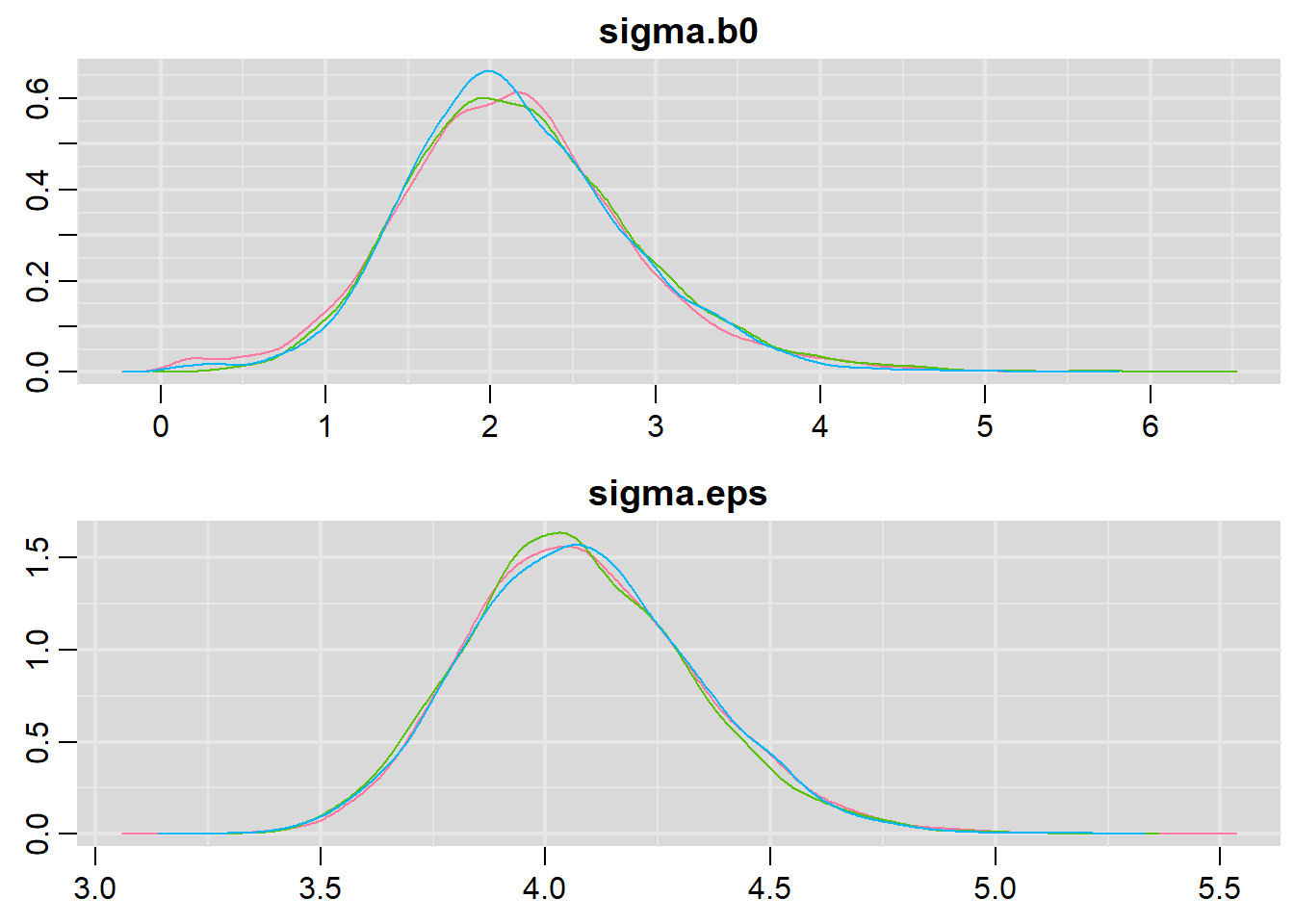
18.15.2 Random intercept and slope model
When specifying mixed models that include multiple random effects (e.g., site-specific intercepts and slopes), we have to consider how these parameters vary and co-vary. In the simple random intercept and slope model from Section 18.6.2, we had 4 variance parameters: \(\sigma_{b_0}, \sigma_{b_1}, cov(b_0, b_1)\) (or \(cor(b_0,b_1))\), and \(\sigma_{\epsilon}\). We will need priors for each of these parameters. One option is to specify a uniform distribution for \(cor(b_0, b_1)\) and priors for each of \(\sigma_{b0}, \sigma_{b1}\) and \(\sigma_{\epsilon}\). Together, these priors specify a prior distribution for the \(2 \times 2\) variance/covariance matrix of the random effects, \(\Sigma_b\):
\(\Sigma_b = \begin{bmatrix} \sigma^2_{b_0} & cov(b_0, b_1)\\ cov(b_0, b_1) & \sigma^2_{b1} \end{bmatrix}\)
We can then specify the distribution of the random effects using dmnorm in JAGS, which refers to the multivariate normal distribution. We specify the mean of this distribution using:
B = \(\begin{bmatrix} \beta_{0i} = \beta_0 + b_{0i}\\ \beta_{1i} = \beta_1 + b_{1i} \end{bmatrix}\)
We also need to specify the precision matrix:
Tau.B = \(\Sigma_b^{-1}\).
We demonstrate how to implement this model using JAGS, below:
jags.lme.rc<-function(){

# Priors for the intercepts
 for (i in 1:n.groups){
  # To allow for correlation between alpha[i] and beta1[i], we need to model
  # their joint (multivariate) distribution
    beta0i[i] <- B[i,1] # Random intercepts
    beta1i[i] <- B[i,2] # Random slopes for age
    B[i,1:2]~ dmnorm(B.hat[i,], Tau.B[,]) # distribution of the vector (beta0[i], beta1[i])
    B.hat[i,1]<-beta0 # mean for intercepts
    B.hat[i,2]<-beta1 # mean for slopes
 }

 # Hyperpriors for intercepts and slopes
  beta0 ~ dnorm(0, 0.001)
  beta1 ~ dnorm(0, 0.001)

 # Hyperpriors for Sigma =  var/cov matrix of the slope/intercept parameters
  sigma.b0 ~ dunif(0,100) # sd intercepts
  sigma.b1 ~ dunif(0,100) # sd of slopes
  cor.b0.b1 ~ dunif(-1,1) # correlation among intercepts and slopes
  Sigma.B[1,1]<-pow(sigma.b0,2)
  Sigma.B[2,2]<-pow(sigma.b1,2)
  Sigma.B[1,2]<-cor.b0.b1*sigma.b0*sigma.b1
  Sigma.B[2,1]<-Sigma.B[1,2]

 # Tau = inverse of Sigma (analogous to precision for univariate normal distribution)
  Tau.B[1:2,1:2]<-inverse(Sigma.B[,])

 # Prior for within-site errors
  tau.eps <- 1 / ( sigma.eps * sigma.eps)       # Residual precision
  sigma.eps ~ dunif(0, 100)         # Residual standard deviation

# Likelihood
 for (i in 1:nobs) {
    dbh[i] ~ dnorm(mu[i], tau.eps)
    mu[i] <- beta0i[site[i]] + beta1i[site[i]]*agec[i]
 }
}


# Parameters to estimate
  parameters <- c("beta0", "beta1", "betaoi", "beta1i", "sigma.b0",
                  "sigma.b1", "sigma.eps", "cor.b0.b1")


# Start Gibbs sampling
  out.rc <- jags.parallel(data = jags.data,
                          parameters.to.save=parameters,
                          model=jags.lme.rc,
                          n.thin=1, n.chains=3, n.burnin=100, n.iter=10000)
Below, we compare the output from JAGS and lmer for the random intercept and slope model:
MCMCsummary(out.rc, params=c("beta0", "beta1", "sigma.b0",
                             "sigma.b1", "cor.b0.b1", "sigma.eps"), round=3)
## mean sd 2.5% 50% 97.5% Rhat n.eff
## beta0 16.460 0.617 15.262 16.451 17.718 1.00 6968
## beta1 2.376 0.603 1.247 2.359 3.613 1.00 1301
## sigma.b0 2.009 0.746 0.581 1.976 3.604 1.00 1298
## sigma.b1 1.148 0.683 0.107 1.096 2.659 1.02 737
## cor.b0.b1 0.134 0.479 -0.821 0.169 0.927 1.01 860
## sigma.eps 4.030 0.258 3.561 4.017 4.568 1.00 7246## Linear mixed model fit by REML ['lmerMod']
## Formula: dbh ~ agec + (1 + agec | site)
## Data: pines
##
## REML criterion at convergence: 917.4
##
## Scaled residuals:
## Min 1Q Median 3Q Max
## -1.90307 -0.72242 -0.08194 0.58100 2.93686
##
## Random effects:
## Groups Name Variance Std.Dev. Corr
## site (Intercept) 3.740 1.934
## agec 1.122 1.059 0.25
## Residual 15.631 3.954
## Number of obs: 160, groups: site, 20
##
## Fixed effects:
## Estimate Std. Error t value
## (Intercept) 16.5258 0.5601 29.506
## agec 2.4502 0.4934 4.966
##
## Correlation of Fixed Effects:
## (Intr)
## agec 0.157We see that posterior means for the variance parameters tend to be larger than the estimates from lmer. The posterior medians are closer to the frequentist estimates. The estimated correlation between \(\beta_{0i}\) and \(\beta_{1i}\) also differs considerably between the two methods, but the 95% credible interval for this parameter is quite wide (-0.821, 0.927). Therefore, the data are not very informative with respect to this parameter.
This brings up an important point - if we include additional random effects (e.g., random intercepts associated with additional grouping variables or random slopes associated with additional level-1 covariates), then our covariance matrix describing the random effects will quickly grow in size requiring the estimation of additional variance and covariance parameters. If, for example, we had a second level-1 covariate and wanted to allow each site to have its own coefficient then we would need to estimate 3 variance parameters (1 for the intercept and 2 for the level-1 coefficients) and 3 covariance parameters describing how the intercept co-varies with the level-1 coefficients and how the 2 level-1 coefficients co-vary. Estimation of these variance parameters can be challenging, unless we have a large number of groups (in this case, sites). Bayesian applications also get more complicated as they require specification of a valid prior for the variance-covariance matrix (see e.g., Chung, Gelman, Rabe-Hesketh, Liu, & Dorie, 2015).
One way to simplify the model is to assume the random intercepts vary independently from the random slopes. Using lmer, we can fit this model using the following notation:
## Linear mixed model fit by REML. t-tests use Satterthwaite's method [
## lmerModLmerTest]
## Formula: dbh ~ agec + (1 | site) + (0 + agec | site)
##    Data: pines
##
## REML criterion at convergence: 917.6
##
## Scaled residuals:
##      Min       1Q   Median       3Q      Max
## -1.92349 -0.73821 -0.08194  0.57261  2.87679
##
## Random effects:
##  Groups   Name        Variance Std.Dev.
##  site     (Intercept)  3.539   1.881
##  site.1   agec         1.129   1.063
##  Residual             15.678   3.960
## Number of obs: 160, groups:  site, 20
##
## Fixed effects:
##             Estimate Std. Error      df t value Pr(>|t|)
## (Intercept)  16.4512     0.5506 14.0053  29.878 4.38e-14 ***
## agec          2.4094     0.4898 15.2072   4.919 0.000178 ***
## ---
## Signif. codes:  0 '***' 0.001 '**' 0.01 '*' 0.05 '.' 0.1 ' ' 1
##
## Correlation of Fixed Effects:
##      (Intr)
## agec 0.037
Here, the (0 + agec | site) tells R that we want each site to have its own coefficient for agec, but we want the coefficients to vary independently of the intercept. Fitting this model in JAGS is rather simple and only requires priors for the three variance parameters, \(\sigma_{b_0}\), \(\sigma_{b_1}\), and \(\sigma_{\epsilon}\).
We will later refer to these as random effects, or more specifically, random intercepts.↩
For some interesting viewpoints on this larger topic, see this dynamic ecology blog and counterpoints here and here↩
In Section 18.12, we will discuss other approaches that are often recommended for choosing an appropriate mixed model.↩
It is quite common for users to just say that they fit a “random effect” for variable \(x\); almost always, this means they included a random intercept associated with \(x\)↩
Again, a random trial consists of collecting a data set of the same size as this one, generated in the same way, assuming all assumptions of the model are met, and then analyzed using the same model mixed-model↩
Note, the
re.formargument can also be used to include some, but not all, random effects when models are specified to have multiple random effects.↩Note,
predictis a generic function for generating predictions from different models; behind the scenes, when we usepredictwith a model fit usinglmerorglmer, it actually calls thepredict.merModfunction↩Note that their
estvariable has been renamed asHRestand theirSAvariable has been renamedStudyAreain theData4Ecologistspackage.↩