Chapter 6 Multicollinearity
Learning objectives
- Be able to describe and identify different forms of multicollinearity
- Understand the effects of multicollinearity on parameter estimates and their standard errors
- Be able to evaluate predictors for multicollinearity using variance inflation factors
- Understand some strategies for dealing with multicollinearity
6.1 Multicollinearity
As we noted in Section 3.13.1, predictor variables will almost always be correlated in observational studies. When these correlations are strong, it can be difficult to estimate parameters in a multiple regression model, leading to coefficients with large standard errors. This should, perhaps, not be too surprising given that we have emphasized the interpretation of regression coefficients in a multiple regression model as quantifying the expected change in \(Y\) as we change a focal predictor by 1 unit while holding all other predictors constant. When two variables are highly correlated, changes in one variable tend to be associated with changes in the other, and therefore, our data do not provide much information about how \(Y\) changes in response to changes in only one of the predictors.
To address this issue, ecologists commonly compute pairwise correlations between all predictor variables and drop one member of any pair when the absolute value of the associated correlation coefficient, \(|r|\) is greater than 0.7 (Dormann et al., 2013). Although pairwise correlations may identify pairs of variables that are collinear (i.e., highly correlated), ecologists should also be concerned with situations in which the information in a predictor variable is largely redundant with the information contained in a suite of predictors (i.e., multicollinearity). Multicollinearity implies that one of the explanatory variables can be predicted by the others (using a linear model) with a high degree of accuracy, and thus has little additional information to provide about how \(Y\) changes when included in a model with the variables that predict it well.
There are several types of collinearity/multicollinearity that can arise when analyzing data. In some cases, we may have multiple measurements that reflect some latent (i.e. unobserved) quantity; Dormann et al. (2013) refers to this as intrinsic collinearity. For example, biologists may quantify the size of their study animals using multiple measurements (e.g., length from head to tail, neck circumference, etc). It would not be surprising to find that pairwise correlations between these different measurements are large because they all relate to one latent quantity, which is overall body size. In other cases, quantitative variables may be constructed by aggregating categorical variables (e.g., percent cover associated with different land-use categories in different pixels within a Geographical Information System [GIS]). These compositional variables must sum to 1, and thus, the last category is completely determined by the others. This is an extreme example of multicollinearity; statistical software will be unable to estimate separate coefficients for each compositional variable along with an overall intercept. Collinearity can also occur structurally, e.g., when fitting models with polynomial terms or with predictors that have very different scales. For example, the correlation between \(x\) and \(x^2\) will often be large (see below).
## [1] 0.9688484This type of collinearity can often be fixed by using various transformations of the explanatory variables (e.g., using orthogonal polynomials as discussed in Section 4.10 or by centering and scaling variables; Schielzeth, 2010). Lastly, variables may be correlated due to other reasons that are harder to identify on their own - e.g., perhaps several predictors covary spatially leading to mild to severe multicollinearity. As an example, temperature, precipitation, and elevation may all co-vary along an elevation gradient. Lastly, collinearity can also happen by chance in small data sets; Dormann et al. (2013) calls this incidental collinearity and suggests it is best addressed through proper sampling or experimental design (e.g., to ensure that predictor variables do not substantially covary).
Some of the symptoms of multicollinearity include:
- variables may be significant in simple linear regression models but not in regression models with multiple predictors as they compete to explain the same variance in \(Y\).
- parameter estimates may have large standard errors, representing large uncertainty, despite large sample sizes
- the p-values associated with t-tests for the individual coefficients in the regression model may be large (\(> 0.05\)), but a multiple degree-of-freedom F test of the null hypothesis that all coefficients is 0 may have a p-value \(<0.05\). In essence, we can conclude that the suite of predictor variables explains significant variation in \(Y\), but we are unable to identify the independent contribution of each of the predictors.
- parameter estimates may change in magnitude (and even sign) depending on what over variables are included in the model (e.g., Table 6.1).
- parameter estimates may be unstable; small changes in the data or model structure can change parameter estimates considerably
6.2 Motivating example: what factors predict how long mammals sleep?
To demonstrate some of these issues, let’s briefly explore a popular data set from the openintro package (Çetinkaya-Rundel et al., 2021) containing measurements of the average amount of time different mammals sleep per 24 hour period (Allison & Cicchetti, 1976; Savage & West, 2007).
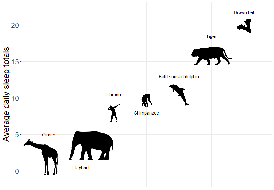
FIGURE 6.1: Average daily sleep totals for several different mammal species. Figure created using images available on PyloPic. Elephant by T. Michael Keesey - CC By 3.0.
Sleep is characterized by either slow wave (non-dreaming) or rapid eye movement (dreaming), with wide variability in the amount of both types of sleep among mammals. In particular, Roe Deer (Capreolus capreolus) sleep < 3 hours/day whereas the Little Brown Bat (Myotis lucifugus) sleeps close to 20 hours per day.
The data set has many possible variables we could try to use to predict sleeping rates, including:
- Lifespan (years)
- Gestation (days)
- Brain weight (g)
- Body weight (kg)
- Predation Index (1-5; 1 = least likely to be preyed upon)
- Exposure Index [1-5: 1 = least exposed (e.g., animal sleeps in a den)]
- Danger Index (1:5, combines exposure and predation; 1= least danger from other animals)
It turns out that all of these variables are negatively correlated with sleep (see the correlations in the first row of Figure 6.2) - no wonder it is so difficult to get a good night’s rest!
library(openintro)
library(dplyr)
data(mammals, package="openintro")
mammals <- mammals %>% dplyr::select(total_sleep, life_span, gestation,
                          brain_wt, body_wt, predation,
                          exposure, danger) %>%
  filter(complete.cases(.))
GGally::ggpairs(mammals)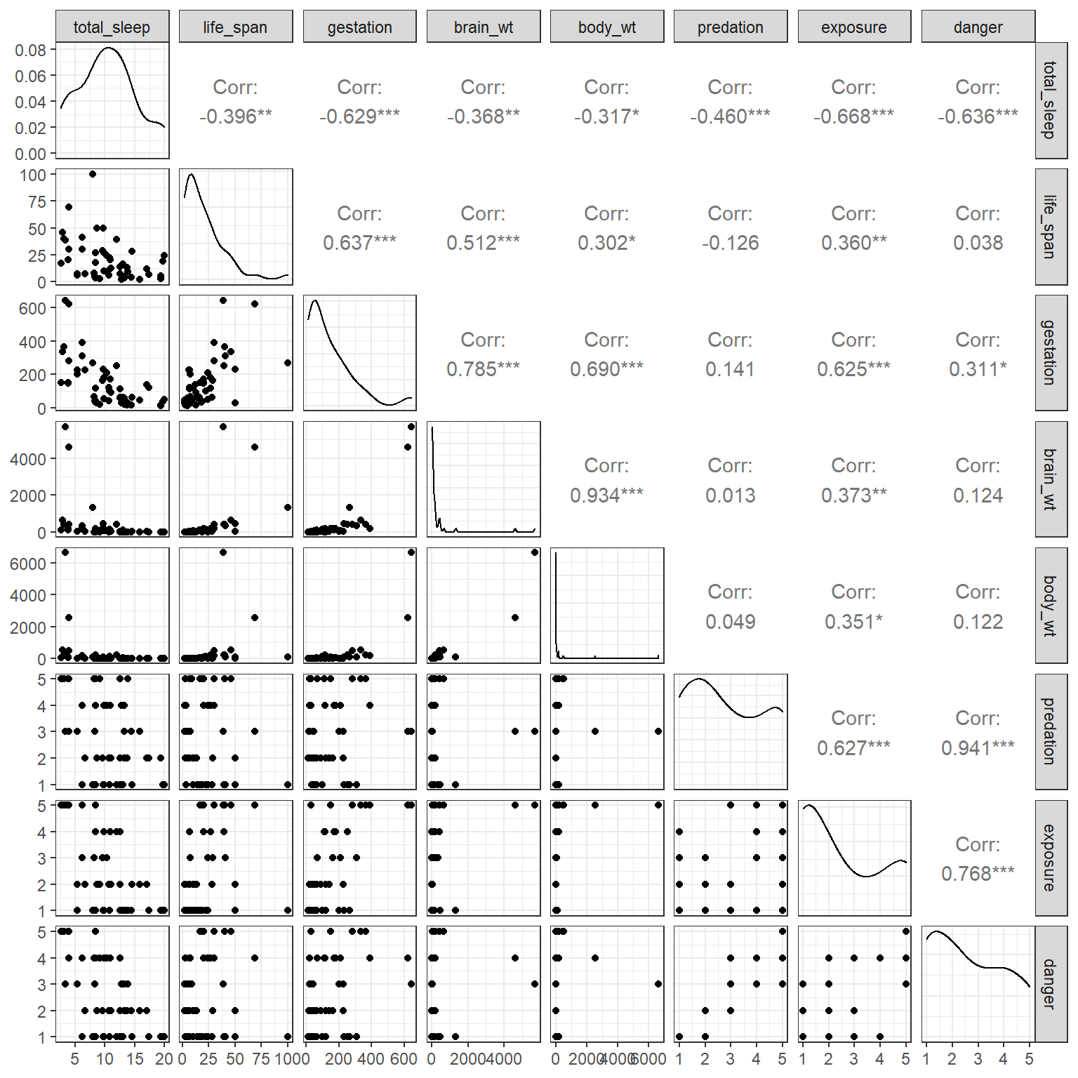
FIGURE 6.2: Scatterplot matrix of the predictors in the mammals data set.
We also see that our predictor variables are highly correlated with each other. Lastly, we see that the distribution of brain_wt and body_wt are severely right skewed with a few large outliers. To reduce the impact of these outliers, we will consider log-transformed predictors, log(brain_wt) and log(body_wt) when including them in regression models19.
To see how this can impact estimated regression coefficients and statistical hypothesis tests involving these coefficients, let’s consider the following two models:
Model 1: Sleep = \(\beta_0 + \beta_1\)life_span
Model 2: Sleep = \(\beta_0 + \beta_1\)life_span \(+ \beta_2\)danger \(+ \beta_3\)log(brain_wt)
model1<-lm(total_sleep ~ life_span, data=mammals)
model2<-lm(total_sleep ~ life_span + danger + log(brain_wt), data=mammals)
modelsummary(list(model1, model2), gof_omit = ".*",
             estimate = "{estimate} ({p.value})",
             statistic = NULL,
             title="Estimates (p-values) for lifespan in a model with and
without other explanatory variables.")| Model 1 | Model 2 | |
|---|---|---|
| (Intercept) | 12.312 (0.000) | 17.837 (0.000) |
| life_span | -0.097 (0.004) | -0.008 (0.811) |
| danger | -1.728 (0.000) | |
| log(brain_wt) | -0.879 (0.001) |
In the first model, life_span is statistically significant and has a coefficient of -0.097 (Table 6.1). However, life_span is no longer statistically significant once we include danger and log(brain_wt), and its coefficient is also an order of magnitude smaller (\(\hat{\beta}_{log.BrainWt} =-0.008\)). What happened?
Because life_span and log(brain_wt) are positively correlated, they will “compete” to explain the same variability in sleep measurements.
[1] 0.7267191If we try to fit a model with all of the explanatory variables, we find that only danger and predation have p-values < 0.05 (Table 6.2). Further, the coefficient for predation is positive despite our intuition that high predation pressure should be negatively correlated with sleep. And, indeed, the coefficient for predation is negative if it is the only explanatory variable in the model. In Sections 6.4 and 7, we will use causal diagrams to explore potential reasons why the magnitude and direction of a regression coefficient may change after adding or excluding a variable.
model3 <- lm(total_sleep ~ life_span + gestation + log(brain_wt) +
               log(body_wt) + predation + exposure + danger, data=mammals)
model4 <- lm(total_sleep ~ predation, data=mammals)
modelsummary(list(model3, model4), gof_omit = ".*",
             estimate = "{estimate} ({p.value})",
             statistic = NULL,
             title="Estimates (p-values) for a model containing all
predictors and one that only contains predation.")| Model 1 | Model 2 | |
|---|---|---|
| (Intercept) | 17.149 (0.000) | 14.465 (0.000) |
| life_span | 0.015 (0.647) | |
| gestation | -0.008 (0.094) | |
| log(brain_wt) | -0.841 (0.189) | |
| log(body_wt) | 0.129 (0.781) | |
| predation | 1.950 (0.046) | -1.448 (0.001) |
| exposure | 0.828 (0.147) | |
| danger | -4.193 (0.001) |
6.3 Variance inflation factors (VIF)
The best way to diagnose collinearity that may involve multiple variables is to calculate a variance inflation factor (VIF), e.g., using the vif function in the car package (Fox & Weisberg, 2019b):
\[\begin{gather} VIF(\hat{\beta}_j) = \frac{1}{1-R^2_{x_j|x_1, ..., x_{j-1}, x_{j+1}, x_p}} \tag{6.1} \end{gather}\]
where \(R^2_{x_j|x_1, ..., x_{j-1}, x_{j+1}, x_p}\) is the multiple \(R^2\) from a regression that predicts \(x_j\) using all other predictors in the model (i.e., lm(\(x_j \sim x_1 + \ldots + x_{j-1} + x_{j+1} + x_p\)). Inspecting equation (6.1), we see that as this \(R^2\) approaches 1, the VIF will approach \(\infty\). The square root of the VIF can be interpreted as providing an indication of how much larger the standard error associated with \(x_j\) is compared to the case where \(x_j\) is uncorrelated with all other predictors (i.e., if \(R^2_{x_j|x_1, ..., x_{j-1}, x_{j+1}, x_p}= 0\)). There are several rules of thumb in the published literature that suggest VIFs \(\ge\) 4 or 5 warrant further inspection and VIFs \(ge\) 10 are particularly problematic (Kutner, Nachtsheim, & Neter, 2004). In an influential paper published in Ecology, Graham (2003) highlighted that a VIF around 2 was high enough to impact the choice of predictor variables when applying common model selection algorithms. In the sections that follow, we will briefly explore the impact of collinearity using a simulation study and then consider the data and examples from Graham (2003) .
Let’s have a look at the VIFs for the sleep data if we were to include all of the predictors. We will use the vif function in the car package to calculate the VIFs:
##     life_span     gestation log(brain_wt)  log(body_wt)     predation
##      2.507122      2.971837     16.568907     13.903451     12.978738
##      exposure        danger
##      5.121031     16.732626
We can also use the check_model function in the performance package to create a nice visualization of the VIFS (Figure 6.3):
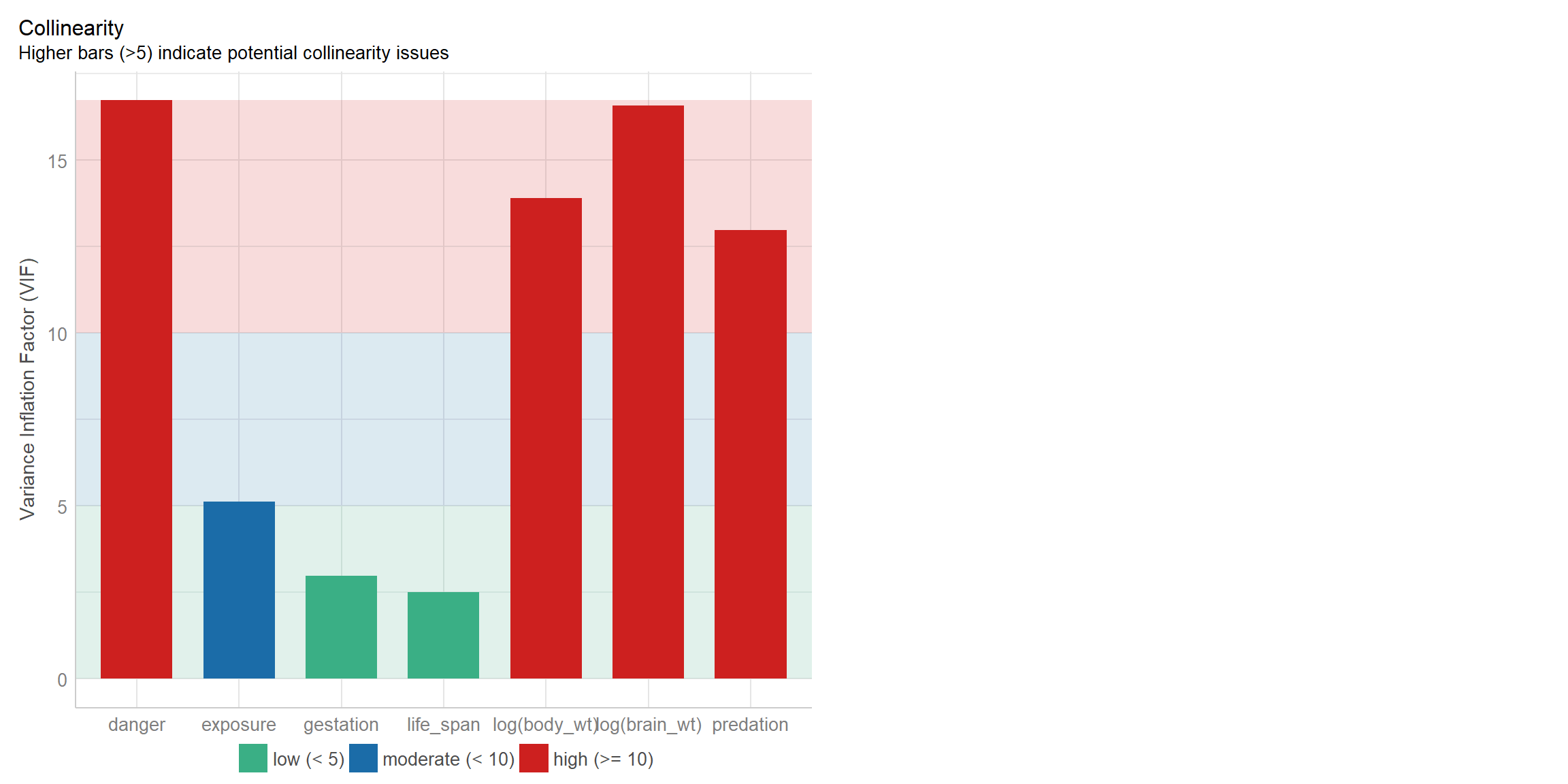
FIGURE 6.3: Variance inflation factors visualized using the check_model function in the performance package (Lüdecke et al., 2021).
We see that several of the VIFs are large and greater than 10, suggesting that several of our predictor variables are collinear. You will have a chance to further explore this data set as part of an exercise associated with this Section.
6.4 Understanding confounding using DAGs: A simulation example
Lets consider a system of variables, represented using a directed acylical graph (DAG)20, below (Figure 6.4), in which arrows represent causal effects:
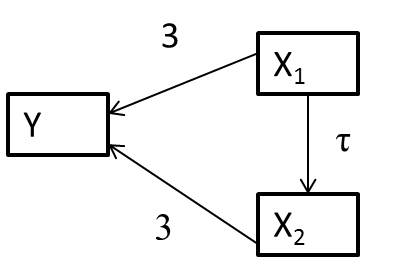
FIGURE 6.4: Directed acyclical graph (DAG) with magnitudes of coefficients depicting causal relationships between x1, x2, and y.
The arrows between \(x_1\) and \(y\) and \(x_2\) and \(y\) indicate that if we manipulate either \(x_1\) or \(x_2\) these changes will have a direct impact on \(y\). The link between \(x_1\) and \(x_2\) also highlights that when we manipulate \(x_1\) we will also change \(x_2\). Thus, \(x_1\) also has an indirect effect on \(y\) that is mediated by \(x_2\) through the path \(x_1 \rightarrow x_2 \rightarrow y\).
I simulated data consistent with the DAG in Figure 6.4, assuming:
- \(X_{1,i} \sim U(0,10)\), where \(U\) is a uniform distribution, meaning that \(X_{1,i}\) can take on any value between 0 and 10 with equal probability.
- \(X_{2,i} =\tau X_{1,i} + \gamma_i\) with \(\gamma_i \sim N(0, 4)\)
- \(Y_i = 10 + 3X_{1,i} + 3X_{2,i} + \epsilon_i\) with \(\epsilon_i \sim N(0,2)\)
I simulated 2000 data sets for values of \(\tau\) ranging from 0 to 9 by 3, and for each data set, I fit the following 2 models:
lm(y ~ x1)lm(y ~ x1 + x2)
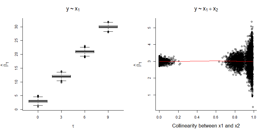
FIGURE 6.5: Results of fitting models with and without \(x_2\) to data simulated using the DAG from Figure 6.4.
We see that:
- the coefficient for \(x_1\) is biased whenever \(x_2\) is not included in the model (unless \(\tau=0\), in which case \(x_1\) and \(x_2\) are independent; left panel of Figure 6.5)
- the magnitude of the bias increases with the correlation between \(x_1\) and \(x_2\) (i.e., with \(\tau\))
- the coefficient for \(x_1\) is unbiased when \(x_2\) is included, but the standard error increases when \(x_1\) and \(x_2\) are highly correlated (right panel of Figure 6.5).
To understand these results, note that:
\[\begin{equation} \begin{split} Y_i = 10 + 3X_{1,i} + 3X_{2,i} + \epsilon_i \text{ and } X_{2,i} =\tau X_{1,i} + \gamma_i \\ \nonumber Y_i = 10 + 3X_{1,i} + 3(\tau X_{1,i} + \gamma_i) + \epsilon_i \\ \nonumber Y_i = 10 + (3+3\tau)X_{1,i} + (3\gamma_i + \epsilon_i) \nonumber \end{split} \end{equation}\]
Thus, when we leave \(x_2\) out of the model, \(x_1\) will capture both the direct effect of \(x_1\) on \(y\) as well as the indirect effect of \(x_1\) on \(y\) that occurs through the path \(x_1 \rightarrow x_2 \rightarrow y\). The relative strength of these two effects are dictated by the coefficients that capture the magnitude of the causal effects along each path. The magnitude for the path \(x_1 \rightarrow y\) is 3 since this is a direct path. For the \(x_1 \rightarrow x_2 \rightarrow y\) path, we have to multiply the coefficients along the path ( \(x_1 \rightarrow x_2\) and \(x_2 \rightarrow y\)), giving \(3\tau\). Thus, the total effect (direct and indirect effect) of manipulating \(x_1\) is given by \(3 + 3\tau\) in this example. We will consider the implications of various causal diagrams in Section 7.
6.5 Alternative strategies for multicollinearity
As we will discuss in Section 8, it paramount to consider how a model will be used when developing strategies for handling messy data situations, including multicollinearity. If our goal is to develop a predictive model, then we may not care about the effect of any one variable in isolation (i.e., we may not be interested in how \(y\) changes as we change \(x_1\) while holding all other variables constant – we just want to be able to predict \(y\) from the suite of available variables). In this case, we may choose to include all variables in our model even if their individual standard errors are inflated due to multicollinearity. We might also choose to include collinear variables if we are interested in estimating causal effects, and we believe that the collinear variables have separate direct effects on the response variable of interest. That is, we may choose to include collinear variables in our model to ensure that we end up with unbiased parameter estimators even if this results in large standard errors for these variables.21 Similarly, we may choose to include variables with high VIFs if they are not of primary interest but need to be included to control for potential confounding of other variables we do care about22.
On the other hand, as alluded to previously, it is common to drop one member of a pair of highly correlated variables. Often users will compare univariate regression models and select the variable that has the higher correlation with the response variable. Alternatively, if one applies a stepwise model selection routine (Section 8.3), it is likely that one of the highly correlated predictors will be dropped during that process because competing predictors will often look “underwhelming” when they are both included. As we will discuss later, such data-driven approaches can lead to overfitting and, as our simulation shows above, they can also lead to biased parameter estimators.
Graham (2003) considers a few other options, including:
- Residual and sequential regression
- Principal components regression
- Structural equation models
We will briefly consider the first two options using the data from Graham (2003) ; structural equation models have a rich history, particularly in the social sciences and deserve their own treatment (by someone more well versed in their use than me!). One option would be Jarrett Byrnes’s course. For a nice introduction, I also suggest reading Grace (2008).
6.6 Applied example: Modeling the effect of correlated environmental factors on the distribution of subtidal kelp
We begin by considering the data from Graham (2003), which are contained in the Data4Ecologists package.
Attaching package: 'Data4Ecologists'The following object is masked from 'package:openintro':
birdsThe data consist of 38 observations with the following predictors used to model the shallow (upper) distributional limit of the subtidal kelp Macrocystis pyrifera.
OD= wave orbital displacement (in meters)BD= wave breaking depth (in meters)LTD= average tidal height (in meters)W= wind velocity (in meters/s).
The distributional limit is contained in a variable named Response. We begin by calculating variance inflation factors for each of the predictor variables:
      OD       BD      LTD        W
2.574934 2.355055 1.175270 2.094319
Next, we use a pairwise scatterplot to explore the relationship among these predictors. Importantly, we do not include the response variable in this plot because we hope to avoid having pairwise correlations between predictor and response variables influence our decisions regarding which predictors to include in our model. Although it is not uncommon to see this type of information used to eliminate some predictor variables from consideration, doing so increases the risk of overfitting one’s data, leading to a model that fits the current data well but fails to predict new data in the future [see Fieberg & Johnson (2015); and Section @(mmi)].
![Pairwise scatterplot of predictor variables in the Kelp data set [@graham2003].](07a-Multicollinearity_files/figure-html/pairs-1.png)
FIGURE 6.6: Pairwise scatterplot of predictor variables in the Kelp data set (Graham, 2003).
We see that all of the variance inflation factors are \(<\) 5, but the correlation between OD and BD is > 0.7 and the correlation between W and OD and W and BD are both > 0.6.
6.7 Residual and sequential regression
Graham (2003) initially considers an approach he refers to as residual and sequential regression, in which variables are prioritized in terms of their order of entry into the model, with higher-priority variables allowed to account for unique as well as shared contributions to explaining the variability of the response variable, \(y\). Although I have not seen this approach applied elsewhere, it is instructive to consider how this approach partitions the variance of \(y\) across a suite of correlated predictors.
Consider a situation in which you are interested in building a model that includes three correlated predictor variables. To apply this approach, we begin by ordering the variables based on their a priori importance, say \(x_1, x_2,\) and then \(x_3\).23 We then construct a multivariable regression model containing the following predictors:
- \(x_1\)
- the residuals of lm(\(x_2 \sim x_1\))
- the residuals of lm(\(x_3 \sim x_1 + x_2\))
In this case, the coefficient for \(x_1\) will capture unique contributions of \(x_1\) to the variance of \(y\) as well as its shared contributions with \(x_2\) and \(x_3\). The coefficient for the residuals of the linear model relating \(x_2\) to \(x_1\) will capture contributions of \(x_2\) to the variance of \(y\) that are unique to \(x_2\) or shared only with \(x_3\) (the coefficient for \(x_1\) is already accounting for any shared contributions of \(x_2\) with \(x_1\)). Lastly, the coefficient for the residuals of the linear model relating \(x_3\) to \(x_1\) and \(x_2\) will capture the contributions of \(x_3\) to the variance of \(y\) that are not shared with \(x_1\) or \(x_2\) and thus unique only to \(X_3\).
For the Kelp data set, Graham (2003) decided on the following order of greatest to least importance, wave orbital displacement (OD), wind velocity (W), average tidal height (LTD), and then wave breaking depth (BD). He then created the following predictors:
  Kelp$W.g.OD<-lm(W~OD, data=Kelp)$resid
  Kelp$LTD.g.W.OD<-lm(LTD~W+OD, data=Kelp)$resid
Kelp$BD.g.W.OD.LTD<-lm(BD~W+OD+LTD, data=Kelp)$resid W.g.OD= to capture the effect ofWthat is not shared withODLTD.g.W.OD= to capture the effect ofLTDthat is not shared withODorWBD.g.W.OD.LTD= to capture the effect ofBDnot shared withOD,W, orLTD
We then fit the model that includes allOD` and all of our derived predictors:
Call:
lm(formula = Response ~ OD + W.g.OD + LTD.g.W.OD + BD.g.W.OD.LTD,
    data = Kelp)

Residuals:
      Min        1Q    Median        3Q       Max
-0.284911 -0.098861 -0.002388  0.099031  0.301931

Coefficients:
               Estimate Std. Error t value Pr(>|t|)
(Intercept)    2.747588   0.078192  35.139  < 2e-16 ***
OD             0.194243   0.028877   6.726 1.16e-07 ***
W.g.OD         0.008082   0.003953   2.045   0.0489 *
LTD.g.W.OD    -0.055333   0.141350  -0.391   0.6980
BD.g.W.OD.LTD -0.004295   0.021137  -0.203   0.8402
---
Signif. codes:  0 '***' 0.001 '**' 0.01 '*' 0.05 '.' 0.1 ' ' 1

Residual standard error: 0.1431 on 33 degrees of freedom
Multiple R-squared:  0.6006,    Adjusted R-squared:  0.5522
F-statistic: 12.41 on 4 and 33 DF,  p-value: 2.893e-06
To interpret the coefficients, we need to keep in mind how the predictors were constructed. For example, we would interpret the coefficient for OD as capturing unique contributions of OD as well as its shared contributions with W, LTD and BD. We would interpret the coefficient for W.g.OD as capturing the unique contributions of W as well as its shared contributions with LTD and BD that are not already accounted for by OD. The non-significant coefficients for LTD.g.W.OD and BD.g.W.OD.LTD could be interpreted as suggesting that the variables LTD and BD offer little to no new information about Response that is not already accounted for by OD and W.
Because of the way we created the variables, the variables are orthogonal - i.e., they are all uncorrelated. Thus, we can eliminate the lesser priority variables without changing the coefficients for the other variables.
               Estimate  Std. Error   t value     Pr(>|t|)
(Intercept) 2.747587774 0.076148241 36.082091 2.796476e-29
OD          0.194243475 0.028122800  6.906975 5.038589e-08
W.g.OD      0.008082141 0.003849614  2.099468 4.305538e-02
The ability to capture unique and shared contributions of multiple correlated variables using orthogonal predictor variables is one of the strengths of the method. The main downside is that the coefficients depend on how we prioritize the predictors as we are unable to separate out their shared and unique contributions.
6.8 Principal components regression
Another way to create orthogonal predictors is to perform a principal component analysis (PCA) on the set of predictor variables under consideration. A PCA will create new orthogonal predictors from linear combinations24 of the original correlated variables:
\(pca_1 = \lambda_{1,1}X_1 + \lambda_{1,2}X_2 + \ldots \lambda_{1,p}x_p\)
\(pca_2 = \lambda_{2,1}X_1 + \lambda_{2,2}X_2 + \ldots \lambda_{2,p}x_p\)
\(\cdots\)
\(pca_p = \lambda_{p,1}X_1 + \lambda_{p,2}X_2 + \ldots \lambda_{p,p}x_p\), where
where \(p\) is the number of original correlated predictors and also the number of new predictors that are orthogonal. These new predictors, \(pca_i\), are often referred to as principal component scores. The \(\lambda\)’s, often referred to as loadings, are unique to each \(pca_i\) and weight the contribution of each of the original variables when forming the new orthogonal variables.
Whereas the sequential regression approach from the last section created new orthogonal predictors through a prioritization and residual regression algorithm, a PCA creates new predictors such that \(pca_1\) accounts for the greatest axis of variation in \((x_1, x_2, ..., x_p)\), \(pca_2\) accounts for greatest axis of remaining variation in \((x_1, x_2, ..., x_p)\), not already accounted for by \(pca_1\), etc25. Because of the way these variables are created, we might expect most of the information in the suite of variables will be contained in the first few principal components. PCAs are relatively easy to visualize in the 2-dimensional case (i.e., \(p=2\); see Figure 6.7)); the first principle component will fall upon the axis with the greatest spread, and the second principle component will fall perpendicular (orthogonal) to the first. This logic extends to higher dimensions but visualization is not longer so easy. When \(p > 2\), it is common to plot just the first two principal components along with vectors that highlight the contributions of the original variables to these principal components (i.e., their loadings on the first two principal components); this type of plot is often referred to as a bi-plot (Figure 6.8).
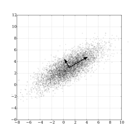
FIGURE 6.7: PCA of a set of bivariate Normal random variables showing the axes associated with the first two principle components. From https://commons.wikimedia.org/wiki/File:GaussianScatterPCA.svg.
There are lots of functions in R that can be used to implement a PCA. Here, we use the princomp function in R (R Core Team, 2021). PCAs formed using the covariance matrix of the predictor data will depend heavily on how variables are scaled (remember, we are finding linear combinations of the original predictor data that explain the majority of the variance in our predictors. If we do not scale our predictors first, or use the correlation matrix, then our principal components will be dominated by the variables that are largest in magnitude as these will have the largest variance). Thus, to avoid these issues, we add the argument cor=TRUE to indicate that we want to form PCAs using the correlation matrix (which effectively scales all predictors to have mean 0 and standard deviation of 1) rather than use the covariance matrix of our predictor variables.
Importance of components:
                          Comp.1    Comp.2     Comp.3     Comp.4
Standard deviation     1.6016768 0.8975073 0.60895215 0.50822166
Proportion of Variance 0.6413421 0.2013799 0.09270568 0.06457231
Cumulative Proportion  0.6413421 0.8427220 0.93542769 1.00000000
We see that the first principal component accounts for 64% of the variation in the predictors, the second principle component accounts for 20% of the variation, and the other two together account for less than 10% of the variation. We can also look at the loadings, which give the \(\lambda\)’s used to create our 4 principal components. The blank values are not 0 but just small (< 0.001), and the signs here are arbitrary (i.e., we could multiply all loadings in a column by -1 and not change the proportion of variance explained by the \(pca\)).
##
## Loadings:
##     Comp.1 Comp.2 Comp.3 Comp.4
## OD   0.548  0.290  0.159  0.768
## BD   0.545  0.179  0.581 -0.577
## LTD -0.338  0.934
## W    0.536  0.110 -0.795 -0.259
##
##                Comp.1 Comp.2 Comp.3 Comp.4
## SS loadings      1.00   1.00   1.00   1.00
## Proportion Var   0.25   0.25   0.25   0.25
## Cumulative Var   0.25   0.50   0.75   1.00
The new PCA variables are contained in pca$scores. We could also calculate these by “hand” if we first scaled and centered our original predictor data and then multiplied those values by the loadings as demonstrated below:
   #scores by "hand" compared to scores returned by princomp
   head(scale(as.matrix(Kelp[,2:5]))%*%pcas$loadings, n = 3)
Comp.1 Comp.2 Comp.3 Comp.4
[1,] -0.1912783 -1.752736 0.66278941 -0.24694830
[2,] 0.6223409 -2.502387 -0.18091063 -0.46900655
[3,] -1.3326878 -0.919048 0.03361542 0.05590063 Comp.1 Comp.2 Comp.3 Comp.4
1 -0.1938459 -1.7762635 0.67168631 -0.25026319
2 0.6306949 -2.5359779 -0.18333907 -0.47530223
3 -1.3505770 -0.9313847 0.03406665 0.05665101As mentioned previously, it is common to plot the two principal component scores along with the loadings, e.g., using the biplot function in R (Figure 6.8). From this plot, we can see that the first principal component is largely determined by OD, BD and W, whereas the second principal component is mostly determined by LTD.
![Bi-plot showing the first two principal components using the Kelp data set [@graham2003], along with the loadings of the original variables.](07a-Multicollinearity_files/figure-html/bi-1.png)
FIGURE 6.8: Bi-plot showing the first two principal components using the Kelp data set (Graham, 2003), along with the loadings of the original variables.
It is important to recognize that \(pca_1\) explains the greatest variation in \((x_1, x_2, ..., x_p)\) and not necessarily the greatest variation in \(y\) (the same goes for the other \(pca_i\)s). Thus, Graham (2003) suggests that all principal components should be included in a regression model. However, it is also common to only include a subset of principal component scores when building regression models (i.e., one of the main reasons to use principal components is to reduce the number of predictor variables included in a model; Harrell Jr, 2015). In this example, the last two principle components account for little variation in the original predictors, so it is unlikely that they will explain much of the variation in \(y\). Still, let’s begin by including all 4 principal component scores:
  Kelp<-cbind(Kelp, pcas$scores)
  lm.pca<-lm(Response~ Comp.1 + Comp.2 + Comp.3 + Comp.4, data=Kelp)
  summary(lm.pca)
Call:
lm(formula = Response ~ Comp.1 + Comp.2 + Comp.3 + Comp.4, data = Kelp)

Residuals:
      Min        1Q    Median        3Q       Max
-0.284911 -0.098861 -0.002388  0.099031  0.301931

Coefficients:
            Estimate Std. Error t value Pr(>|t|)
(Intercept)  3.24984    0.02321 140.035  < 2e-16 ***
Comp.1       0.09677    0.01449   6.678 1.33e-07 ***
Comp.2       0.02931    0.02586   1.134    0.265
Comp.3      -0.03564    0.03811  -0.935    0.356
Comp.4       0.07722    0.04566   1.691    0.100
---
Signif. codes:  0 '***' 0.001 '**' 0.01 '*' 0.05 '.' 0.1 ' ' 1

Residual standard error: 0.1431 on 33 degrees of freedom
Multiple R-squared:  0.6006,    Adjusted R-squared:  0.5522
F-statistic: 12.41 on 4 and 33 DF,  p-value: 2.893e-06
Since the \(pca_i\)’s are orthogonal, the coefficients will not change if we drop some of the \(pca_i\)’s (as demonstrated below):
##
## Call:
## lm(formula = Response ~ Comp.1, data = Kelp)
##
## Residuals:
##      Min       1Q   Median       3Q      Max
## -0.28269 -0.09537  0.00437  0.06927  0.35765
##
## Coefficients:
##             Estimate Std. Error t value Pr(>|t|)
## (Intercept)  3.24984    0.02385 136.265  < 2e-16 ***
## Comp.1       0.09677    0.01489   6.499 1.51e-07 ***
## ---
## Signif. codes:  0 '***' 0.001 '**' 0.01 '*' 0.05 '.' 0.1 ' ' 1
##
## Residual standard error: 0.147 on 36 degrees of freedom
## Multiple R-squared:  0.5398, Adjusted R-squared:  0.527
## F-statistic: 42.23 on 1 and 36 DF,  p-value: 1.507e-07
Thus, in the end, we may choose to capture the combined effect of OD, W, LTD and BD using a single principal component (and 1 model degree of freedom). The main downside of this approach is that the principal components can be difficult to interpret as it is a function of all of these variables.
6.9 Other methods
There are several other multivariate regression techniques that one could consider when trying to eliminate collinear variables. In particular, one might consider combining similar variables (e.g., “weather variables”) using a PCA or variable clustering or scoring technique that creates an index out of multiple variables (e.g., weather severity formed by adding a 1 whenever temperatures are below or snow depth above pre-defined thresholds; DelGiudice, Riggs, Joly, & Pan, 2002; Dormann et al., 2013; Harrell Jr, 2015). Scoring techniques are not that different from a multiple regression model, except rather than attempt to estimate optimal weights associated with each predictor (i.e., separate regression coefficients), variables are combined by assigning a +1, 0, -1 depending on whether each the value of each predictor is expected to be indicative of larger or smaller values of the response variable, and then a single coefficient is estimated.26 There are also several statistical methods (e.g., factor analysis, partial least squares, structural equation models, etc) that use latent variables to represent various constructs (e.g., personality, size, etc) that can be informed by or are the products of multiple correlated variables. We will not discuss these here, but note that they are popular in the social sciences. Some of these methods are touched on in Dormann et al. (2013).
Sometimes researchers will state that predictors were log-transformed to make them Normally distributed. Linear regression models do NOT assume that predictors are Normally distributed, so this reasoning is faulty. However, it is sometimes beneficial to consider log-transformations for predictor variables that have skewed distributions as a way to reduce the influence of individual outlying observations.↩
We will talk more about DAGs in Section 7, but for now, note that a DAG displays causal connections among a set of variables↩
It may sound strange to you to see “parameter estimator” here rather than “parameter estimates”. However, note that in statistics, bias is defined in terms of a difference between a fixed parameter and the average estimate across repeated samples (i.e., the mean of a sampling distribution). Thus, bias is associated with the method of generating estimates (i.e., the estimator), not the estimates themselves.↩
Another approach that is sometimes used is ridge regression (Hoerl & Kennard, 1970; Dormann et al., 2013), which adds a constant to elements of the correlation matrix when estimating parameters. Ridge regression estimators accept a small amount of bias to improve precision.↩
Graham (2003) suggests this ordering can be based on one’s instincts, intuition, or prior or current data, but how to use this information when deciding upon an order is not discussed in detail.↩
As a reminder, a linear combination is a weighted sum of the predictors.↩
We can decompose \(\Sigma\), the correlation matrix of \((x_1, x_2, ..., x_p)\) using \(\Sigma = V\Lambda V^T\) where \(V\) is a \([n \times p]\) matrix of eigenvectors, equivalent to the principal components, and \(\Lambda\) is a diagonal matrix of eigenvalues↩
Jacob Cohen, a famous statistician, argued that we might be better off using these indices directly for inference rather than regression models when faced with a small number of observations and many correlated predictors; Cohen (1992)↩