Chapter 2 Bootstrapping
Learning objectives
- To understand how a bootstrap can be used to quantify uncertainty, particularly when assumptions of linear regression may not be met.8
- To further your coding skills by implementing a cluster-level bootstrap appropriate for certain types of data sets containing repeated observations.
Zuur et al. (2009) lead off their immensely popular book, Mixed Effects Models and Extensions in Ecology with R, with the statement (p. 19), “In Ecology, the data are seldom modeled adequately by linear regression models. If they are, you are lucky.” Modern statistical methods, such as generalized linear models and random effects models, allow one to relax the assumptions of normality, constant variance, and independence that constrain the applicability of linear regression. Most of this book will be devoted to these more modern methods For now, however, we will explore how we can use a different tool, bootstrapping, to quantify uncertainty when the assumptions of linear regression do not hold. The bootstrap is also a useful approach for understanding the concept of a sampling distribution, because it requires us to repeatedly generate and analyze data sets to quantify how parameter estimates vary across multiple sampling events (see Fieberg, Vitense, & Johnson, 2020 for further discussion and examples).
2.1 Motivating data example: RIKZ [Dutch governmental institute] data
We will consider a data set from Zuur et al. (2009) containing abundances of \(\sim\) 75 invertebrate species measured on various beaches along the Dutch Coast. The data were originally published in Janssen & Mulder (2004) and Janssen & Mulder (2005). The pictures, below, were sent to me by Professor Gerard Janssen who did some of the field sampling.
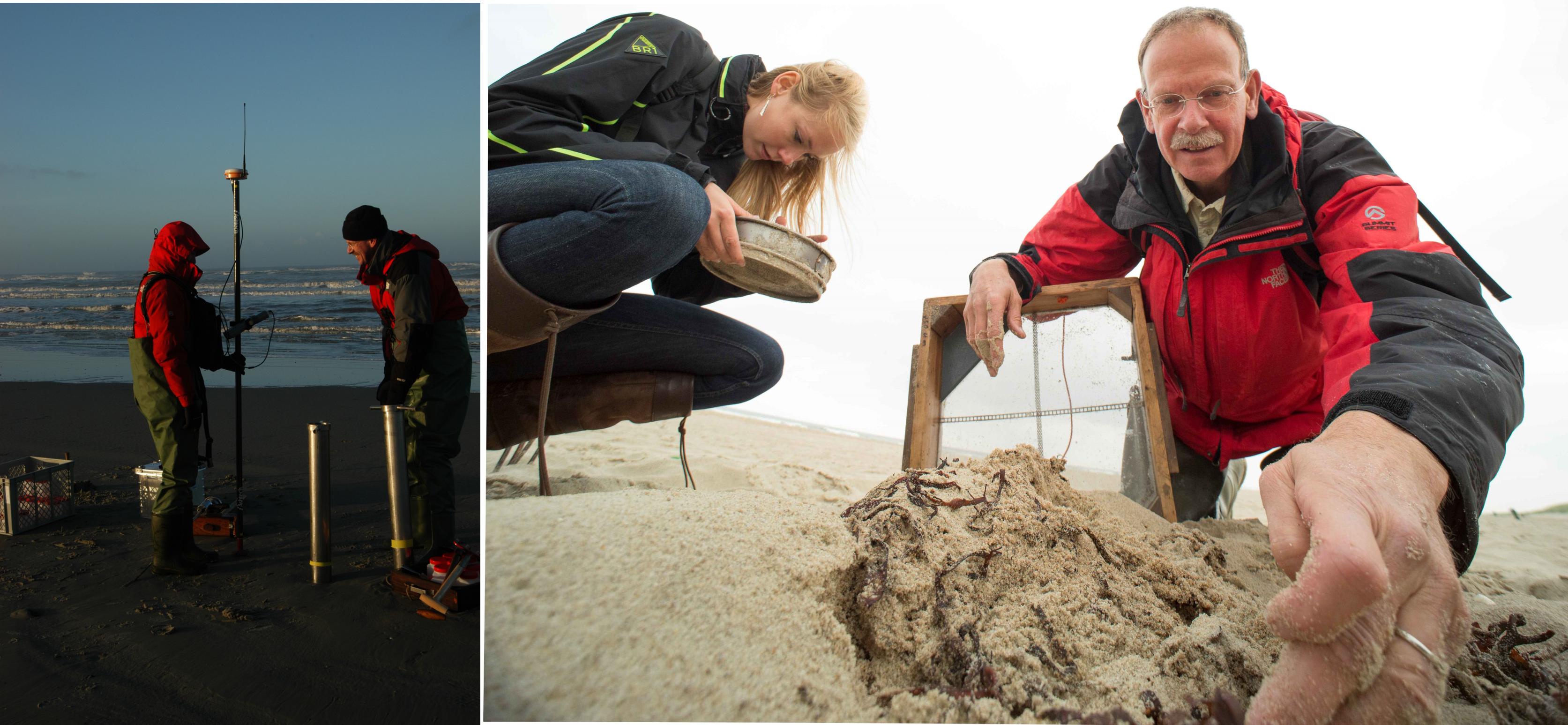
FIGURE 2.1: Photos provided by Dr. Gerard Janssen who led the field sampling associated with the RIKZ data set.
The data, which can be accessed via the Data4Ecologists library, were collected at 5 stations at each of 9 beaches. The beaches were located at 3 different levels of exposure to waves (high, medium, or low). For now, we will focus on the following variables:
Richness= species richness (i.e., the number of species counted).NAP= height of the sample site (relative to sea level). Lower values indicate sites closer to or further below sea level, which implies more time spent submerged.Beach= a unique identifier for the specific beach where the observation occurred
We will load the data, turn Beach into a factor variable, and plot Richness versus NAP:
ggplot(RIKZdat, aes(NAP, Richness)) +
  geom_point() +
  geom_smooth(method = "lm", formula = y ~ x,  se = FALSE) + xlab("NAP") +
  ylab("Richness")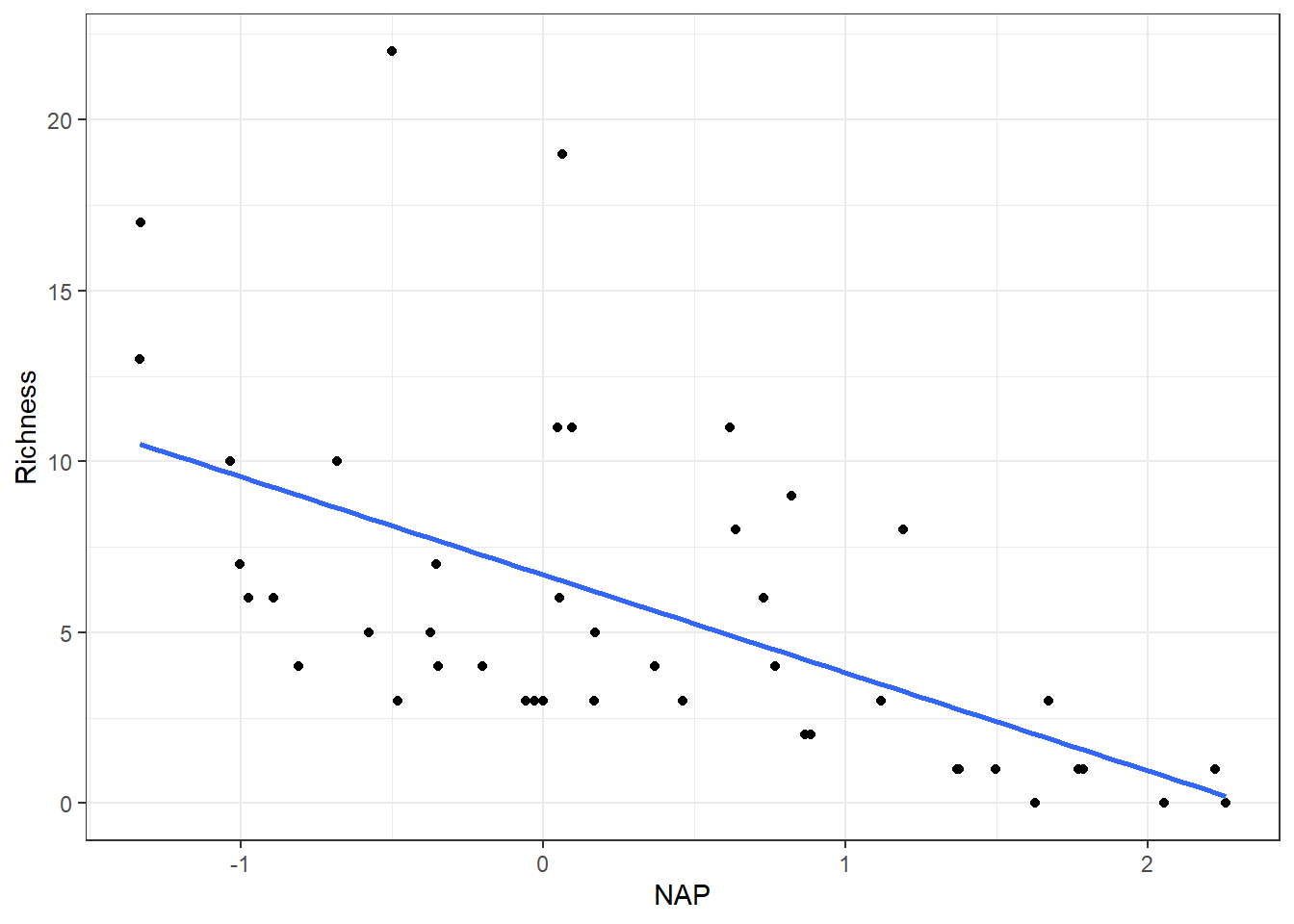
FIGURE 2.2: Species richness versus NAP for data collected from 9 beaches in the Netherlands.
The line seems to do a fairly good job of capturing the general pattern. Below is the output from running a linear regression to determine the best-fit line in the plot above.
Call:
lm(formula = Richness ~ NAP, data = RIKZdat)

Residuals:
    Min      1Q  Median      3Q     Max
-5.0675 -2.7607 -0.8029  1.3534 13.8723

Coefficients:
            Estimate Std. Error t value Pr(>|t|)
(Intercept)   6.6857     0.6578  10.164 5.25e-13 ***
NAP          -2.8669     0.6307  -4.545 4.42e-05 ***
---
Signif. codes:  0 '***' 0.001 '**' 0.01 '*' 0.05 '.' 0.1 ' ' 1

Residual standard error: 4.16 on 43 degrees of freedom
Multiple R-squared:  0.3245,    Adjusted R-squared:  0.3088
F-statistic: 20.66 on 1 and 43 DF,  p-value: 4.418e-05
As we might have suspected from the scatterplot, there is an indication that there is a significant, negative linear relationship between the two variables. But we should make sure our assumptions hold before we trust the standard errors and p-values.
Recall, simple linear regression models can be described using the following equations:
\[Y_i = \beta_0 + \beta_1X_i + \epsilon_i\]
\[\epsilon_i \sim N(0, \sigma^2)\]
Think-pair-share: Which of the following assumptions do you think are met based on the output from the model?
Assumptions:
- Homogeneity of variance (constant scatter above and below the line); i.e., \(var(\epsilon_i) = \sigma^2\) (a constant)
- Independence: Correlation\((\epsilon_i, \epsilon_j) = 0\) for all \(i \ne j\).
- Linearity: \(E[Y_i \mid X] = \beta_0 + X_i\beta_1\)
- Normality: \(\epsilon_i\) come from a Normal (Gaussian) distribution
The answer is probably “none of the above!” Lets look at residual plots using the resid_panel function in the ggResidPanel package (Goode & Rey, 2019):
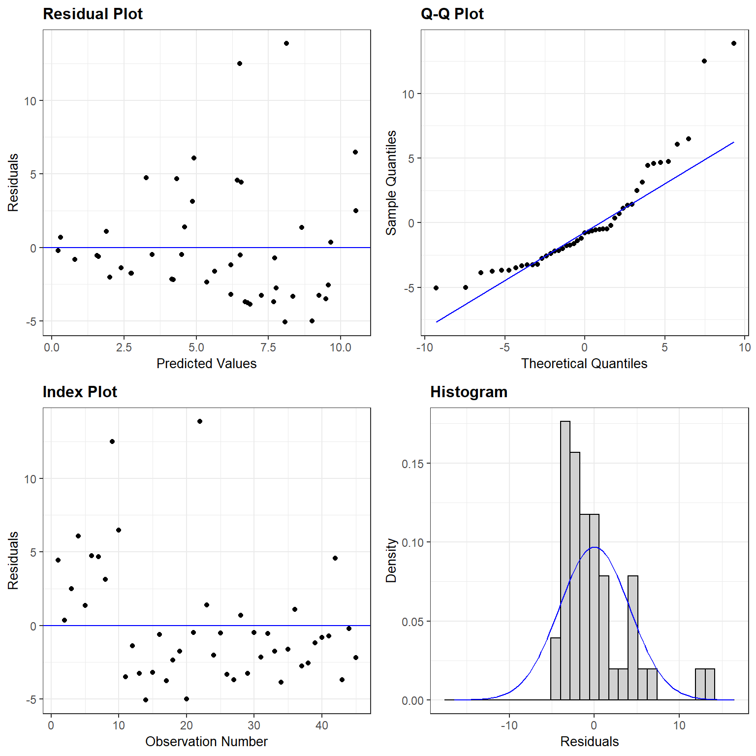
FIGURE 2.3: Residual plots for the linear regression model relating species Richness to NAP in the RIKZdat data set formed using the resid_panel function in the ggResidpanel package (Goode & Rey, 2019).
Homogeneity of variance: the plot of residuals versus fitted values shows a clear increase in variance as we move from left to right (i.e., from smaller to larger predicted values).
Gaussian distribution: the histogram of the residuals suggests they are right-skewed rather than Normally distributed, and the Q-Q plot shows notable deviations from the Q-Q line.
Linearity: the average value of Richness at any given value of NAP looks like it is fairly well described by the line. But, what happens when NAP gets large? If we extrapolate outside of the range of the data, then our line will predict negative values of Richness which is clearly not possible.
Independence: observations are probably not independent since we collected five observations from each beach. Any two observations from the same beach are likely to be more alike than two observations from two different beaches (even after accounting for the effect of NAP). The index plot shows that the first ten observations (from beaches 1 and 2) all had positive residuals, whereas most of the residuals for the other three beaches are negative.
2.2 Consequences of assumption violations
The regression coefficients in a linear regression model are estimated by minimizing the sums of squared deviations between observations and the fitted line:
\(\hat{\beta}\) minimizes: \(\sum_{i=1}^{n}(Y_i-[\beta_0+ X_i\beta_1])^2\).
Least-squares can be motivated from just the linearity and independence assumptions. The linearity assumption seems reasonable over the range of the data, so as long as we do not extrapolate outside the range of our data, we may be OK with this assumption. But, what are the consequences of other assumption violations?
Homogeneity of variance: Least squares assigns equal weight to all observations. If our observations are independent, and our model for the mean is correct, then equal weighting of observations should not introduce bias into our estimates of \(\beta\). However, other weighting schemes can result in more precise estimates (i.e., estimates that vary less from sample to sample). Approaches like generalized least squares (Section 5) and generalized linear models (Section 14) assign more weight to observations in regions of predictor space that are less variable.
Normality: This assumption is needed to derive the sampling distribution of \(\frac{\hat{\beta}}{SE(\hat{\beta})}\). Without this assumption, the sampling distribution of our estimators9 does not follow a t-distribution, and thus, the p-values for the hypothesis tests associated with the intercept and slope may not be accurate. However, the Central Limit Theorem tells us that the sampling distribution of least-squares estimators will converge to that of a Normal distribution as our sample size moves towards infinity. Differences between the t-distribution and Normal distribution also become negligible as the the sample size increases. Therefore, violations of the Normality assumption may not be too consequential if samples sizes are large.
Independence: The main consequence of having non-independent data is that our SE’s for \(\hat{\beta}\) will typically be too small, confidence intervals too narrow, and p-values too small. When data are naturally grouped or “clustered” in some way, we will have less information than we would have if we were able to collect an equally-sized data set in which all observations are independent. We will often refer to groups that share unmeasured characteristics (e.g., observations from the same beach) as clusters.
Again, the rest of this book will be about developing model-based solutions to allow for non-Normal, clustered data.
If we at least can conclude a linear model is still appropriate for describing the relationship between the average species Richness and NAP, then we can still use least squares to estimate \(\beta_0\) and \(\beta_1\); however, we need a different way to calculate our standard errors, calculate confidence intervals, and conduct hypothesis tests – we need a method that works well even when our data are not independent or Normally distributed. One option may be to use a bootstrap to quantify uncertainty.
2.3 Introduction to the Bootstrap
Lets return to the idea of a sampling distribution from Section 1. We can visualize the process of generating a sampling distribution from multiple samples of data, all of the same size and taken from the same population, and then calculating the same statistic from each data set (in our case, \(\hat{\beta}\)) - see Figure 2.4 from Fieberg et al. (2020).
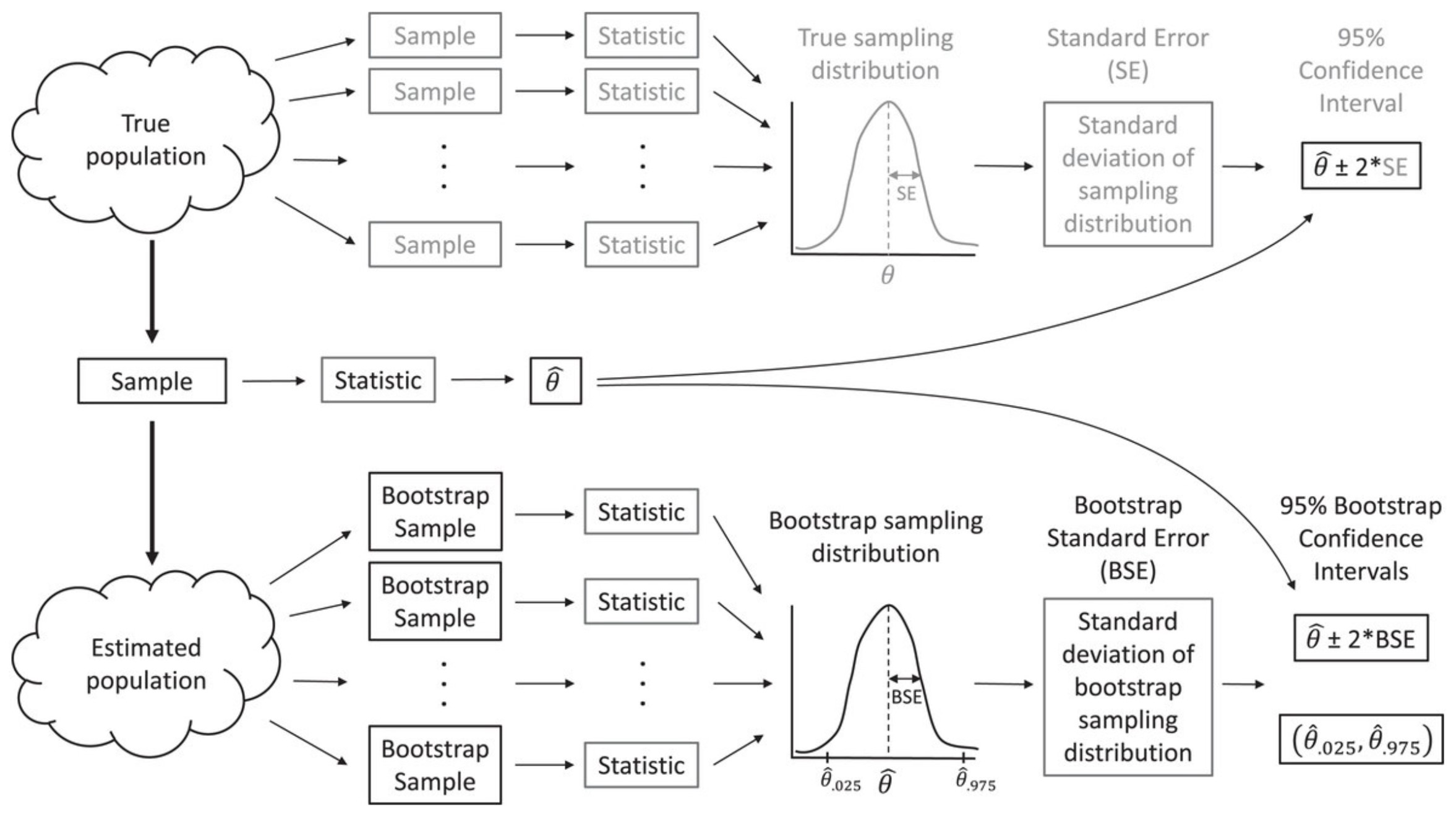
FIGURE 2.4: The bootstrap allows us to estimate characteristics of the sampling distribution (e.g., its standard deviation) by repeatedly sampling from an estimated population. Figure from Fieberg, J. R., Vitense, K., and Johnson, D. H. (2020). Resampling-based methods for biologists. PeerJ, 8, e9089. DOI: 10.7717/peerj.9089/fig-2
If all of our assumptions hold, we know:
\[\frac{\hat{\beta}-\beta}{SE(\hat{\beta})} \sim t_{n-2}\]
However, this will not be the case if our assumptions do not hold. Further, we cannot derive the sampling distribution like we did in Section 1 if we are uncomfortable with these assumptions about the true data-generating process (DGP). What do we mean by the data-generating process? The assumed data-generating process describes our assumptions about what the population looks like and also the mechanisms by which we observe a sample of observations from the population. In the linear model, the assumed DGP has the following characteristics:
- the values of \(Y_i\) at any given value of \(X_i\) are normally distributed with mean \(\mu_i = \beta_0 + \beta_1X_i\) and variance \(\sigma^2\).
- the sample values of \(Y_i\) and \(X_i\) that we observe are independent and representative of the larger population of values
If we are uncomfortable making these assumptions, what can we do? We might try changing our assumption about the DGP. For example, we might just want to just stick with the second assumption - i.e., that the data we have are independent and representative of the larger population of \((X_i, Y_i)\) pairs. Or, perhaps we assume the clusters of observations from the different beaches are independent and representative of the clusters of observations that make up the population. This leads us to the concept of a non-parametric bootstrap.
Bootstrapping provides a way to estimate the SE of a statistic (in this case, \(\hat{\beta}\)) by resampling our original data with replacement. Essentially, we are using the distribution of values in our sample data as an estimate of the distribution of values in the population. Then, by 1) repeatedly resampling our data with replacement and 2) calculating the same statistic for each of these generated data sets, we can approximate the sampling distribution of our statistic under a DGP where the primary assumption is that our sample observations are independent and representative of the larger population.
2.3.1 Bootstrap procedure
If our sample data are representative of the population, as we generally assume when we have a large number of observations selected by simple random sampling, then we can use the distribution of values in our sample to approximate the distribution of values in the population. For example, we can make many copies of our sample data and use the resulting data set as an estimate of the whole population. With this estimated population in place, we could repeatedly sample from it, calculate the statistic for each of these sampled data sets, and then compute the standard deviation of these sample statistics to form our estimated standard error. In practice, we do not actually need to make multiple copies of our sample data to estimate the population; instead, we form new data sets by sampling our sample data with replacement, which effectively does the same thing. This means that each observation in the original data set can occur zero, one, two, or more times in the generated data set, whereas it occurred exactly once in the original data set.
This process allows us to determine how much our estimates vary across repeated samples. We quantify this variability using the standard deviation of our estimates across repeated samples and refer to this standard deviation as our bootstrap standard error (SE).
A bootstrap sample is a random sample taken with replacement from the original sample, of the same size as the original sample – a “simulated” new sample, in a sense.
A bootstrap statistic is the statistic of interest, such as the mean or slope of the least-squares regression line, computed from a bootstrap sample
A bootstrap distribution is the distribution of bootstrap statistics derived from many bootstrap samples.
Whereas the sampling distribution will typically be centered on the population parameter, the bootstrap distribution will typically be centered on the sample statistic.10 That is OK, what we really want from a bootstrap distribution is a measure of variability from sample to sample. The variability of the bootstrap statistics should be similar to the variability of sample statistics in a sampling distribution (if we could actually repeatedly sample from the population) – the spread of the bootstrap and sampling distributions should be very similar even if their centers are not. Thus, we can estimate the standard error using the standard deviation of the bootstrap distribution.
2.3.2 Bootstrap example: Simple linear regression
To demonstrate the bootstrap, let’s revisit the LionNoses data set from Section 1. We will calculate a 95% confidence interval for the intercept and slope parameters using a bootstrap, which we will then compare to standard t-based confidence intervals for these parameters. To generate the bootstrap confidence interval, we will:
- Generate a bootstrap data set by resampling our original observations with replacement.
- Calculate our bootstrap statistics, \(\hat{\beta}_0\) and \(\hat{\beta}_1\), by fitting a linear model to our bootstrap data set.
We will repeat steps 1 and 2 a large number of times to form our bootstrap distribution, which we then plot:
set.seed(08182007)
library(abd)
data("LionNoses")
nboot <- 10000 # number of bootstrap samples
nobs <- nrow(LionNoses)
bootcoefs <- matrix(NA, nboot, 2)
for(i in 1:nboot){
  # Create bootstrap data set by sampling original observations w/ replacement
  bootdat <- LionNoses[sample(1:nobs, nobs, replace=TRUE),]
  # Calculate bootstrap statistic
  lmboot <- lm(age ~ proportion.black, data = bootdat)
  bootcoefs[i,] <- coef(lmboot)
}
par(mfrow = c(1, 2))
hist(bootcoefs[,1], main = expression(paste("Bootstrap distribution of ", hat(beta)[0])), xlab = "")
hist(bootcoefs[,2], main = expression(paste("Bootstrap distribution of ", hat(beta)[1])), xlab = "")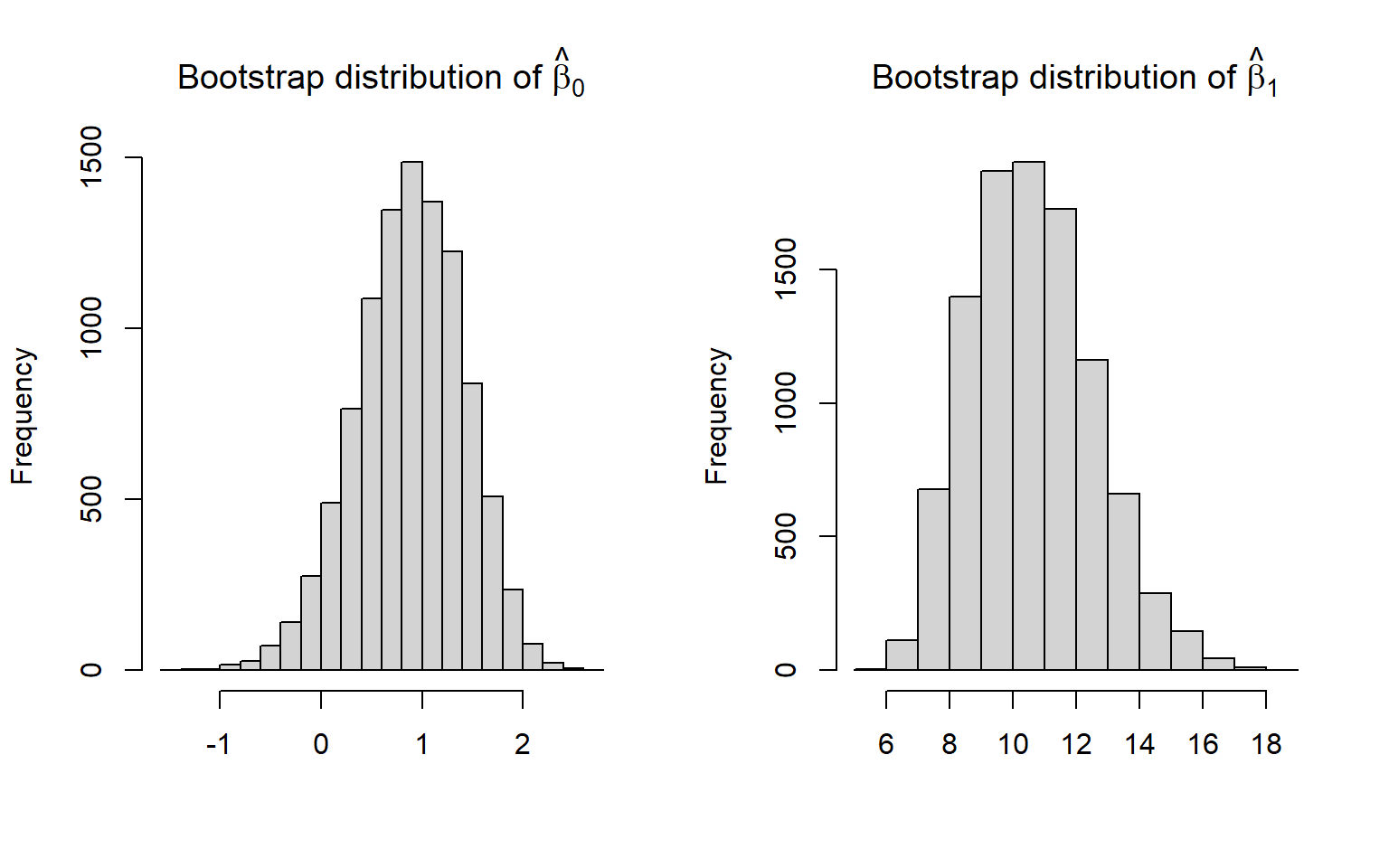
FIGURE 2.5: Bootstrap distribution of regression coefficients relating the age of lions to the proportion of their nose that is black.
The bootstrap distributions are relatively bell-shaped and symmetric, so we could use a Normal approximation to generate confidence intervals for the intercept and slope parameters. To do so, we would calculate the bootstrap standard error as the standard deviation of the bootstrap statistics. We would then take our original sample statistics \(\pm 1.96 SE\). Alternatively, we could use percentiles of the bootstrap distribution to calculate a confidence interval. We demonstrate these two approaches, below, and compare them to the standard t-based interval.
# Fit the model to the original data to get our estimates
lmnoses <- lm(age ~ proportion.black, data = LionNoses)

# Calculate bootstrap standard errors
se<-apply(bootcoefs, 2, sd)

# Confidence intervals
# t-based
confdat.t <- confint(lmnoses)
# bootstrap normal
confdat.boot.norm <- rbind(c(coef(lmnoses)[1] - 1.96*se[1], coef(lmnoses)[1] + 1.96*se[1]),
                           c(coef(lmnoses)[2] - 1.96*se[2], coef(lmnoses)[2] + 1.96*se[2]))
# bootstrap percentile
confdat.boot.pct <- rbind(quantile(bootcoefs[,1], probs = c(0.025, 0.975)),
                          quantile(bootcoefs[,2], probs = c(0.025, 0.975)))

# combine and plot
confdats <- rbind(confdat.t, confdat.boot.norm, confdat.boot.pct)
confdata <- data.frame(LCL = confdats[,1],
                       UCL = confdats[,2],
                       method = rep(c("t-based", "bootstrap-Normal", "bootstrap-percentile"),
                                    each=2),
                       parameter = rep(c("Intercept", "Slope"), 3))
confdata$estimate <- rep(coef(lmnoses),3)
ggplot(confdata, aes(y = estimate, x = " ", col = method)) +
  geom_point() +
  geom_pointrange(aes(ymin = LCL, ymax = UCL),  position = position_dodge(width = 0.9)) +
  facet_wrap(~parameter, scales="free") +xlab("")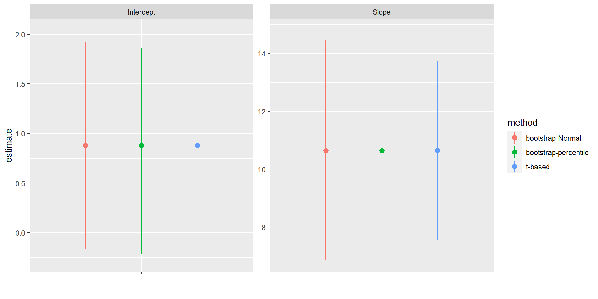
FIGURE 2.6: Comparison of t-based and bootstrap intervals for the intercept and slope of the regression relating the age of lions to the proportion of their nose that is black.
For this particular example, we see that the bootstrap confidence intervals are slightly narrower than the t-based interval for the intercept and slightly wider for the slope. Thus, we pay a small price, in terms of precision, if we are unwilling to make certain assumptions about the DGP (e.g., the residuals are normally distributed with constant variance) and go with the bootstrap confidence interval for the slope instead. For bell-shaped bootstrap distributions, Normal-based and percentile-based bootstrap confidence intervals often work well and will usually give similar results. For small samples or skewed bootstrap distributions, however, better methods exist and should be considered (see e.g., Davison & Hinkley, 1997; Hesterberg, 2015; Puth, Neuhäuser, & Ruxton, 2015).
2.4 Replicating the sampling design
When we use a bootstrap, we are explicitly assuming that it captures the main features of the DGP that resulted in our original sample data. Thus, bootstrap sampling should mimic the original sampling design. What do we do if we have clustered data (i.e., multiple observations taken from the same sampling unit, such as a beach)? Assuming “clusters” are independent from one another (e.g., knowing the \(\epsilon\) for an observation at beach 1 tells us nothing about the likely \(\epsilon\) for an observation at beach 2), we can resample clusters with replacement (keeping all observations associated with the cluster). The number of clusters in the bootstrap sample should be the same as in the original sample.
Visually, this corresponds to:
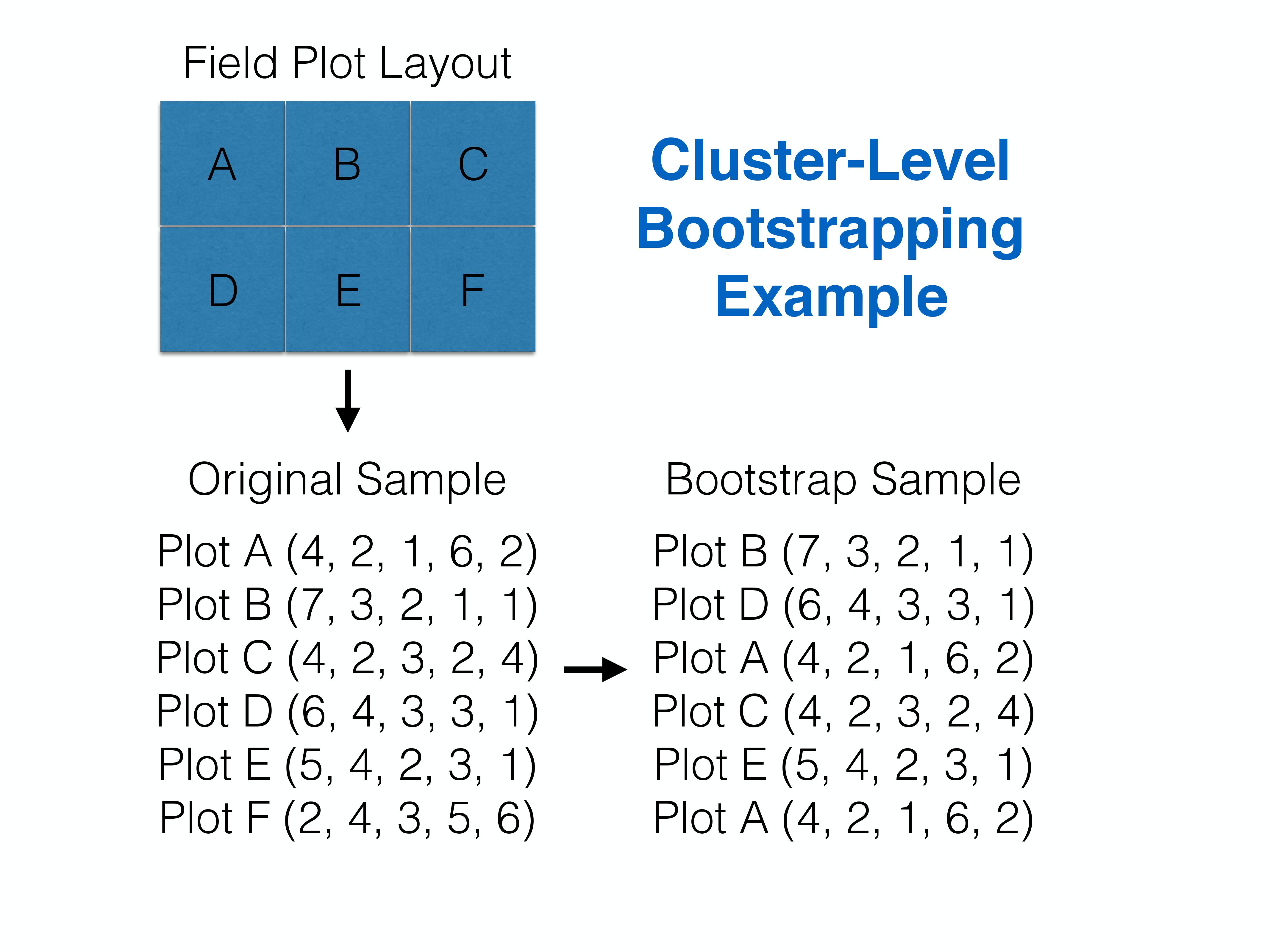
FIGURE 2.7: Cluster-level bootstrapping resamples whole clusters of observations with replacement. Figure constructed by Althea Archer.
Important caveats: The cluster-level bootstrap that is described above works best when we have balanced data (all clusters have the same number of observations; in this case we have five observations at each beach). This approach may be sub-optimal when applied to unbalanced data and potentially problematic depending on the mechanisms causing variability in sample sizes among clusters (e.g., if the size of the cluster is in some way related to the response of interest; Williamson, 2014). In addition, this approach makes the most sense when we are interested in the effect of predictor variables that do not vary within a cluster (Fieberg et al., 2020). One of the homework exercises associated with this chapter asks you to implement this approach by resampling beaches with replacement. Example code for generating a single bootstrap sample in this case is given below.
# let's use the bootstrap to deal with non-constant variance and clustering
# Determine the number of unique beaches
uid<-unique(RIKZdat$Beach)
nBeach<-length(uid)

# Single bootstrap, draw nBeaches with replacement from the
# original pool of beaches
(bootids<-data.frame(Beach=sample(uid, nBeach, replace=T)))
Beach
1 3
2 7
3 7
4 1
5 3
6 5
7 4
8 2
9 2
 1  2  3  4  5  6  7  8  9
 5 10 10  5  5  0 10  0  0
2.5 Utility of the bootstrap
There are 2 primary reasons why you may want to consider a bootstrap. The first is that you may want to make fewer assumptions about the underlying GDP, particularly when assumptions of common statistical methods (e.g., Normally, constant variance) do not seem appropriate. The second reason is that you may be interested in estimating uncertainty associated with a parameter or a function of one or more parameters for which an analytical expression for the standard error is not available. To highlight this latter point, consider that analytical expressions for the standard error are available for many estimators of the parameters you encounter in an introductory statistics class:
- the sample mean as an estimator of the population mean: SE\((\bar{x})\) = \(\frac{\sigma}{\sqrt{n}}\)
- the sample proportion as an estimator of the population proportion: SE\((\hat{p})\) = \(\sqrt{\frac{p(1-p)}{n}}\)
- the slope of the least-squares regression line: SE\((\hat{\beta}_1)\) = \(\frac{\sqrt{\sum_{i=1}^n (y_i - \hat{y}_i)^2 / (n -2)}}{\sqrt{\sum_{i=1}^n(x_i- \bar{x})^2}}\)
But what if you want to estimate the uncertainty with \(1/\beta_1\)? Or, you want to fit a mechanistic model of growth to weight-at-age data (see Section 10.6), and need to calculate uncertainty with the predicted weight at any given age, which is given by a non-linear function of your parameters (\(L_{\infty}, K, t_0\)) = \(L\infty \left(1- e^{-K(Age - t_0)}\right)\)? You will not find an analytical expression for the standard error in either of these cases, but you can always use the bootstrap to estimate a confidence interval. Two other interesting applications of the bootstrap include estimating model-selection uncertainty (Section 8.7.2) and uncertainty associated with clades on a phylogenetic tree (Felsenstein, 1985 ; Efron, Halloran, & Holmes, 1996).
Later, we will see other options for calculating uncertainty intervals for parameters and functions of parameters estimated using maximum likelihood (Section 10.5, Section 10.7.1, Section 10.9) or using Bayesian methods of inference (Section 11). It is extremely useful to become comfortable with at least one of these approaches.
There are several ways to use bootstrapping to quantify uncertainty associated with regression models. Here we will consider a specific method that uses case resampling.↩
An estimator is a method of generating an estimate of an unknown parameter from observed data.↩
When this is not the case, the bootstrap can be used to estimate estimator bias.↩