Chapter 3 Multiple regression
Learning Objectives
- Understand how to specify regression models using matrix notation.
- Become familiar with creating dummy variables to code for categorical predictors
- Interpret the results of regression analyses that include both categorical and quantitative variables
- Understand approaches for visualizing the results of multiple regression models
3.1 Introduction to multiple regression
So far, we have considered regression models containing a single predictor, often referred to as simple linear regression models. In this section, we will consider models that contain more than one predictor. We can again write our model of the data generating process (DGP) in two ways:
\[\begin{gather} Y_i = \beta_0 + \beta_1X_{i,1} + \beta_2X_{i,2} + \ldots + \beta_p X_{i,p} + \epsilon_i \quad (i = 1, \ldots, n) \nonumber \\ \epsilon_i \sim N(0, \sigma^2) \nonumber \end{gather}\]
Or:
\[\begin{gather} Y_i \sim N(\mu_i, \sigma^2) \nonumber \\ \mu_i = \beta_0 + \beta_1X_{i,1} + \beta_2X_{i,2} + \ldots + \beta_p X_{i,p} \quad (i = 1, \ldots, n) \nonumber \end{gather}\]
The above expressions define linear regression models in terms of individual observations. It will also be advantageous, at times, to be able to define the model for all observations simultaneously using matrices. Doing so will provide insights into how models are represented in statistical software, including models that allow for non-linear relationships between predictor and response variables (Section 4). In addition, matrix notation will provide us with a precise language for describing uncertainty associated with the predictions of linear models. Use of matrix notation will be important for:
- understanding methods for calculating uncertainty in \(\hat{\mu}_i = \hat{\beta}_0 + \hat{\beta}_1X_{i,1} + \hat{\beta}_2X_{i,2} + \ldots \hat{\beta}_p X_{i,p}\) (we glossed over this in Section 1.8 where we showed code for calculating confidence and prediction intervals in regression but did not provide equations or derive expressions for these interval estimators).
- specifying models for observations that are not independent (e.g., Section 5 and Section 18).
3.2 Matrix notation for regression
Let’s start by writing our linear regression model as:
\[\begin{gather} Y_i = \beta_0 + \beta_1X_i + \epsilon_i \quad (i = 1, \ldots, n) \nonumber \\ \epsilon_i \sim N(0, \sigma^2) \nonumber \end{gather}\]
This implies:
\[\begin{eqnarray*} Y_1 & = & \beta_0 + \beta_1X_1 + \epsilon_1 \\ Y_2 & = & \beta_0 + \beta_1X_2 + \epsilon_2 \\ & \vdots & \\ Y_n & = & \beta_0 + \beta_1X_n + \epsilon_n \end{eqnarray*}\]
Alternatively, We can write this set of equations very compactly using matrices:
\[\begin{equation*} \begin{bmatrix}Y_1 \\ Y_2 \\ \vdots \\ Y_n \end{bmatrix} = \begin{bmatrix}1 & X_1 \\ 1 & X_2 \\ \vdots & \vdots \\ 1 & X_n \end{bmatrix} \times \begin{bmatrix} \beta_0 \\ \beta_1 \end{bmatrix} + \begin{bmatrix} \epsilon_1 \\ \epsilon_2 \\ \vdots \\ \epsilon_n \end{bmatrix} \end{equation*}\]
or
\[\begin{gather} Y_{[n\times1]} = X_{[n\times 2]}\beta_{[2\times 1]} + \epsilon_{[n\times 1]} \nonumber \end{gather}\]
We can multiply two matrices, \(A\) and \(B\), together if the number of columns of the first matrix is equal to the number of rows in the second matrix. Let the dimensions of \(A\) be \(n \times m\) and the dimension of \(B\) be \(m \times p\). Matrix multiplication results in a new matrix with the number of rows equal to the number of rows in \(A\) and number of columns equal to the number of columns in \(B\), i.e., the matrix will be of dimension \(n \times p\). The \((i, j)\) entry of this matrix is formed by taking the dot product of row \(i\) and column \(j\), where the dot product is the sum of element-wise products (Figure 3.1).
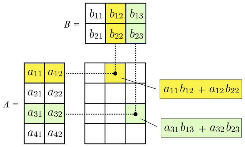
FIGURE 3.1: Matrix multiplication by Svjo – CC BY-SA 4.0..
Using matrix notation, we can generalize our model to include any number of predictors (shown below for \(p-1\) predictors):
\[\begin{equation*} \begin{bmatrix}Y_1 \\ Y_2 \\ \vdots \\ Y_n \end{bmatrix} = \begin{bmatrix}1 & X_{11} & X_{12} & \cdots & X_{1,p-1} \\ 1 & X_{21} & X_{22} & \cdots & X_{2,p-1} \\ \vdots & \vdots & \vdots & & \vdots \\ 1 & X_{n1} & X_{n2} & \cdots & X_{n,p-1} \end{bmatrix} \times \begin{bmatrix} \beta_0 \\ \beta_1 \\ \vdots \\ \beta_{p-1} \end{bmatrix} + \begin{bmatrix} \epsilon_1 \\ \epsilon_2 \\ \vdots \\ \epsilon_n \end{bmatrix} \end{equation*}\]
\[\begin{equation*} Y_{[n\times1]} = X_{[n\times p]}\beta_{[p\times 1]} + \epsilon_{[n\times 1]} \end{equation*}\]
The matrix, \(X\), is referred to as the design matrix and encodes all of the information present in our predictors. In this Section, we will learn how categorical variables and interactions are represented in the design matrix. It Section 4, we will learn how various methods for modeling non-linearities linearities in the relationship between our predictors and our dependent variable can be represented in a design matrix.
It is also useful to know how we can write our alternative formulation of the linear regression model using matrix notation. Specifically, we can write:
\[\begin{equation} \begin{split} Y \sim N(X\beta, \Sigma) \end{split} \end{equation}\]
Here, \(\Sigma\) is an \(n \times n\) variance covariance matrix. Its diagonal elements capture the variances of the observations and the off-diagonal elements capture covariances. Under the assumptions of linear regression, our observations are independent (implying the covariances are 0) and have constant variance, \(\sigma^2\). Thus:
\[\Sigma_{n \times n} = \begin{bmatrix} \sigma^2 & 0 & 0 & \cdots & 0\\ 0 & \sigma^2 & 0 & \cdots & 0 \\ 0 & 0 & \sigma^2 & \cdots & 0 \\ \vdots & \vdots & \vdots & \ddots & \vdots \\ 0 & 0 & 0 & \cdots & \sigma^2 \end{bmatrix} = \sigma^2 I_{[n \times n]}, \text{ where } I_{[n \times n]} = \begin{bmatrix} 1 & 0 & 0 & \cdots & 0\\ 0 & 1 & 0 & \cdots & 0 \\ 0 & 0 & 1 & \cdots & 0 \\ \vdots & \vdots & \vdots & \ddots & \vdots \\ 0 & 0 & 0 & \cdots & 1 \end{bmatrix}\].
3.3 Parameter estimation, sums-of-squares, and R\(^2\)
We can use lm to find estimates of intercept (\(\beta_0\)) and slope parameters (\(\beta_1, \beta_2, \ldots\)) that minimize the sum of squared differences between our observations and the model predictions:
\(\sum_i^n(Y_i-\hat{Y})^2 = \sum_i^n(Y_i-[\beta_0 + \beta_1X_{1,i} +\beta_2X_{2,i} + \ldots])^2\)
Further, we can again decompose the total variation, quantified by the total sums of squares (SST), into variation explained by the model (SSR) and residual sums of squares (SSE):
- \(SST_{df=n-1} = \sum_i^n(Y_i-\bar{Y})^2\)
- \(SSE_{df=n-p} = \sum_i^n(Y_i-\hat{Y})^2\)
- \(SSR_{df=p-1} = SST-SSE = \sum_i^n(\hat{Y}_i-\bar{Y})^2\)
The Coefficient of Determination (R\(^2\)) is calculated the same way as with simple linear regression (\(R^2 = SSR/SST\)). However, adding additional predictors always increases R\(^2\). Thus, we will eventually also want to consider an adjusted R\(^2\), quantified as:
\[\begin{equation*} R^2_\mathrm{adj} = \frac{\frac{\mathrm{SSR}}{p-1}}{\frac{SST}{n-1}} = \left( \frac{n-1}{p-1}\right) \frac{\mathrm{SSR}}{\mathrm{SST}} \end{equation*}\]
The adjusted-R\(^2\) penalizes for additional predictors and so will not always increase as you add predictors. Thus, it should provide a more honest measure of variance explained, particularly when the model contains many predictors. We will consider this measure in more detail when we compare the fits of multiple competing models (Section 8).
We have the same assumptions (linearity, constant variance, Normality) as we do with simple linear regression and can use the same diagnostic plots to evaluate whether these assumptions are reasonably met.
However, it’s also important to diagnose the degree to which explanatory variables are correlated with each other (a topic we will address in more detail when we cover multicollinearity in Section 6).
3.4 Parameter interpretation: Multiple regression with RIKZ data
Recall the RIKZ data from Section 2. We will continue to explore this data set, assuming (naively) that the observations are independent. Earlier, we fit a model relating species Richness to the height of the sample site relative to sea level, NAP. From our regression results, we can write our estimate of the best-fit line as:
\[\begin{equation} Richness_i=6.886-2.867 NAP_i +\epsilon_i \nonumber \end{equation}\]
What if we also hypothesized that humus (amount of organic material) also influences Richness (in addition to NAP)?
The multiple linear regression model formula would look like:
\[Richness_i = \beta_0 + \beta_1NAP_i + \beta_2Humas_i + \epsilon_i\]
Let’s fit this model in R and compare it to the model containing only NAP.
lmfit1 <- lm(Richness ~ NAP, data = RIKZdat)
lmfit2 <- lm(Richness ~ NAP + humus, data = RIKZdat)
modelsummary(list(lmfit1, lmfit2),
  gof_omit = "^(?!R2)",
  estimate = "{estimate} ({std.error})",
  statistic = NULL,
  title = "Estimates of regression parameters (SE) for regression parameters
in one and two-variable models fit to the RIKZ data.")| Model 1 | Model 2 | |
|---|---|---|
| (Intercept) | 6.686 (0.658) | 5.459 (0.830) |
| NAP | -2.867 (0.631) | -2.512 (0.623) |
| humus | 21.942 (9.710) | |
| R2 | 0.325 | 0.398 |
| R2 Adj. | 0.309 | 0.369 |
We see that the slope for NAP changed slightly (from -2.9 to -2.5) and the adjusted R\(^2\) went from 0.31 to 0.37. Instead of a best-fit line through data in two dimensions, we now have a best fit plane through data in three dimensions (Figure 3.2).
FIGURE 3.2: Visualizing the regression model with 2 predictors. Code was adpoted from https://stackoverflow.com/questions/47344850/scatterplot3d-regression-plane-with-residuals.
Our interpretation of regression parameters is similar to that in simple linear regression, except now we have to consider a change in one variable while holding other variables in the model constant:
- \(\beta_1\) describes the change in
Richnessfor every 1 unit increase inNAPwhile holdingHumusconstant. - \(\beta_2\) describes the change in
Richnessfor every 1 unit increase inHumuswhile holdingNAPconstant. - \(\beta_0\): the level of
RichnessifHumusandNAPare both simultaneously equal 0.
Although it is easy to fit multiple regression models with more than two predictors, we will no longer be able to visualize the fitted model in higher dimensions. Before we consider more complex models, however, we will first explore how to incorporate categorical predictors into our models.
3.5 Categorical predictors
To understand how categorical predictors are coded in regression models, we will begin by making a connection between the standard t-test and a linear regression model with a categorical predictor with two levels or categories.
3.5.1 T-test as a regression
Here, we will consider mandible lengths (in mm) of 10 male and 10 female golden jackals (Canis aureus) specimens from the British Museum (Manly, 1991).

FIGURE 3.3: Golden jackles (Canis aureus) in the Danube Delta, Romania. Image by Andrei Prodan from Pixabay.
males<-c(120, 107, 110, 116, 114, 111, 113, 117, 114, 112)
females<-c(110, 111, 107, 108, 110, 105, 107, 106, 111, 111)
We might ask: Do males and females have, on average, different mandible lengths? Let’s consider a formal hypothesis test and confidence interval for the difference in population means:
\[\begin{equation} H_0: \mu_m = \mu_f \text{ versus } H_a: \mu_m \ne \mu_f \end{equation}\]
where \(\mu_m\) and \(\mu_f\) represent population means for male and female jackals, respectively.
If we assume that mandible lengths are Normally distributed in the population11, and that the variance for male and female jaw lengths are about the same12, then we can use the following code to conduct a t-test for a difference in means:
    Two Sample t-test

data:  males and females
t = 3.4843, df = 18, p-value = 0.002647
alternative hypothesis: true difference in means is not equal to 0
95 percent confidence interval:
 1.905773 7.694227
sample estimates:
mean of x mean of y
    113.4     108.6
We can also conduct this same test using a regression model with sex as the only predictor. First, we will have to create a data.frame with mandible lengths (quantitative) and sex (categorical).
  jaws sex
1  120   M
2  107   M
3  110   M
4  116   M
5  114   M
6  111   M
We can then fit a linear regression model to these data and inspect the output:
Call:
lm(formula = jaws ~ sex, data = jawdat)

Residuals:
   Min     1Q Median     3Q    Max
  -6.4   -1.8    0.1    2.4    6.6

Coefficients:
            Estimate Std. Error t value Pr(>|t|)
(Intercept) 108.6000     0.9741 111.486  < 2e-16 ***
sexM          4.8000     1.3776   3.484  0.00265 **
---
Signif. codes:  0 '***' 0.001 '**' 0.01 '*' 0.05 '.' 0.1 ' ' 1

Residual standard error: 3.08 on 18 degrees of freedom
Multiple R-squared:  0.4028,    Adjusted R-squared:  0.3696
F-statistic: 12.14 on 1 and 18 DF,  p-value: 0.002647
We see that the t value and Pr(>|t|) values for sexM are identical to the t-statistic and p-value from our two-sample t-test. Also, the estimated intercept is identical to the sample mean for females. And, if we look at a confidence interval for the regression parameters, we see that the interval for the sexM coefficient is the same as the confidence interval for the difference in means that is output by the t.test function (and, in fact, the coefficient for sexM is equal to the difference in sample means).
                 2.5 %     97.5 %
(Intercept) 106.553472 110.646528
sexM          1.905773   7.694227
To understand these results, we need to know how R accounts for sex in the model we just fit.
3.5.2 Dummy variables: Reference (or effects) coding
We can use the model.matrix function to see the design matrix that R uses to fit the regression model. Here, we print the 2nd, 3rd, 16th, and 17th rows of this matrix (so that we see observations from both sexes):
##    (Intercept) sexM
## 2            1    1
## 3            1    1
## 16           1    0
## 17           1    0
Let’s also look at the data from these cases:
##    jaws sex
## 2   107   M
## 3   110   M
## 16  105   F
## 17  107   F
We see that R created a new variable, sexM, to indicate which cases are males (sexM = 1) and which are females (sexM = 0). Knowing this allows us to write our model in matrix notation (shown here for these 4 observations):
\[\begin{equation*} \begin{bmatrix}107\\ 105 \\ 107 \\ 107 \\ 106 \\ \vdots \end{bmatrix} = \begin{bmatrix}1 & 1 \\ 1 & 0 \\ 1 & 0 \\ 1 & 0 \\ \vdots & \vdots \end{bmatrix} \times \begin{bmatrix} \beta_0 \\ \beta_1 \end{bmatrix} + \begin{bmatrix} \epsilon_1 \\ \epsilon_2 \\ \epsilon_3 \\ \epsilon_4 \\ \vdots \end{bmatrix} \end{equation*}\]
Think-Pair-Share: How can we estimate \(\mu_m\), the mean jaw length for males, from the fitted regression model?
To answer this question, let’s write our model as:
\[Y_i = \beta_0 + \beta_1I(\mbox{sex=male})_{i} + \epsilon_i\]
\[I(\mbox{sex=male})_{i} = \left\{ \begin{array}{ll} 1 & \mbox{if male}\\ 0 & \mbox{if female} \end{array} \right.\]
Here, I have used the notation I(condition) to indicate that we want to create a variable that is equal to 1 when condition is TRUE and 0 otherwise. In general, we will refer to this type of variable as an indicator variable or, more commonly, a dummy variable.
Using this model description, we can estimate the mean jaw length of males by plugging in a 1 for \(I(\mbox{sex=male})_{i}\):
\[Y_i = \beta_0 + \beta_1(1)\]
I.e., we can estimate the mean jaw length of males by summing the two regression coefficients:
\[\begin{equation*} \hat{Y}_i = 108.6 + 4.8 = 113.4, \end{equation*}\]
which is the mean for males that is reported by the t.test function.
In summary, the default method used to account for categorical variables in R is to use reference or effects coding such that:
- the intercept represents the mean for a reference category (when all other predictors in the model are set to 0)
- dummy or indicator variables represent differences in means between other categories and the reference category.
3.5.3 Dummy variables: Cell means coding
It turns out that there are other ways to code the same information contained in the variable sex, and these different parameterizations lead to the exact same model, but expressed with a different set of coefficients. In this section, we will consider what is often called cell-means or means coding:
\[Y_i = X_{i,m}\beta_m + X_{i,f}\beta_f + \epsilon_i\]
\[X_{i,m} = \left\{ \begin{array}{ll} 1 & \mbox{if the } i^{th} \mbox{ observation is from a male}\\ 0 & \mbox{if from a female} \end{array} \right.\]
\[X_{i,f} = \left\{ \begin{array}{ll} 1 & \mbox{if the } i^{th} \mbox{ observation is from a female}\\ 0 & \mbox{if from a male} \end{array} \right.\]
Because “male” and “female” are mutually exclusive categories so far as these data are concerned13, each individual \(i\) will be either male or female, so either \(X_{i,f}\) or \(X_{i,m}\) will be 1 and the other will be 0, and \(\beta_m\) will represent the mean \(Y\) for males and \(\beta_f\) the mean \(Y\) for females.
In R, we can fit this model using means coding using:
Call:
lm(formula = jaws ~ sex - 1, data = jawdat)

Residuals:
   Min     1Q Median     3Q    Max
  -6.4   -1.8    0.1    2.4    6.6

Coefficients:
     Estimate Std. Error t value Pr(>|t|)
sexF 108.6000     0.9741   111.5   <2e-16 ***
sexM 113.4000     0.9741   116.4   <2e-16 ***
---
Signif. codes:  0 '***' 0.001 '**' 0.01 '*' 0.05 '.' 0.1 ' ' 1

Residual standard error: 3.08 on 18 degrees of freedom
Multiple R-squared:  0.9993,    Adjusted R-squared:  0.9992
F-statistic: 1.299e+04 on 2 and 18 DF,  p-value: < 2.2e-16
The -1 here tells R to remove the column of 1s in our design matrix (which usually represent the intercept). With means coding, our model is parameterized in terms of the two group means rather than using the mean for females and the difference in means between males and females. Note: we cannot have a model with all of these parameters (\(\mu_f, \mu_m\), and \(\mu_m-\mu_f\)) since one of these is completely determined by the other two. The -1 in the formula (jaws ~ sex - 1) tells R not to include an overall intercept, which permits estimation of the second group mean in its place.
3.5.4 Comparing assumptions: Linear model and t-test
What are the assumptions of our model for the jaw lengths? Well, they are the same ones that we have for fitting linear regression models with continuous predictors:
- constant variance of the errors (i.e., the two groups are assumed to have equal variance, \(\sigma^2\))
- the residuals, and by extension, the data within each group, are Normally distributed
These are the same assumptions of the two-sample t-test. Let’s see if they are reasonable:
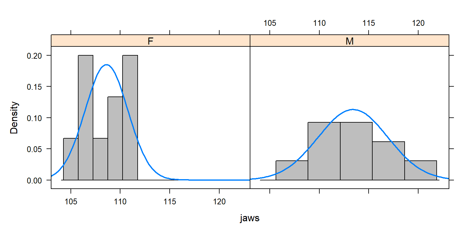
FIGURE 3.4: Evaluating the Normality and constant variance assumptions associated with golden jackal jaw-length data from the British Museum (Manly, 1991).
We have a small data set, so it is difficult to say anything definitively, but it appears that the variance may be larger for males. Later, we will see how we can relax these assumptions using the gls function in the nlme package (see Section 5) and using JAGS (Section 11)
3.6 Categorical variables \(> 2\) levels
To account for differences among \(k\) groups of a categorical variable, we can again use either reference/effects coding or means coding.
3.6.1 Effects coding
With effects coding, we include an overall intercept and \(k-1\) dummy variables. Each dummy variable is used to identify group membership for one of the \(k-1\) groups other than the reference; membership in the \(k^{th}\) group is indicated by having 0’s for all of the other \(k-1\) dummy variables. The intercept will again represent a reference group, and the coefficients for the dummy variables will represent differences between each of the other \(k-1\) categories and the reference group. R will create these dummy variables for us, but understanding how the effects of categorical variables are encoded in regression models will facilitate parameter interpretation and allow us to fit customized models when desired (e.g., see Section 3.7.3). In addition, we will need to create our own dummy variables when fitting models in a Bayesian framework using JAGS (Section 12.4).
Let’s return to the RIKZ data and our model of species Richness. What if we suspected that some species were only present in some weeks such that Richness varied by week in addition to NAP? Let’s see what happens if we add week to the model:
Call:
lm(formula = Richness ~ NAP + week, data = RIKZdat)

Residuals:
    Min      1Q  Median      3Q     Max
-5.2493 -2.4558 -0.7746  1.4261 15.7933

Coefficients:
            Estimate Std. Error t value Pr(>|t|)
(Intercept)   9.0635     1.6291   5.563 1.68e-06 ***
NAP          -2.6644     0.6327  -4.211 0.000131 ***
week         -1.0492     0.6599  -1.590 0.119312
---
Signif. codes:  0 '***' 0.001 '**' 0.01 '*' 0.05 '.' 0.1 ' ' 1

Residual standard error: 4.088 on 42 degrees of freedom
Multiple R-squared:  0.3629,    Adjusted R-squared:  0.3326
F-statistic: 11.96 on 2 and 42 DF,  p-value: 7.734e-05
Since week is coded as an integer (equal to 1, 2, 3 or 4), we see that R assumes it is a continuous predictor and estimates a single coefficient representing the overall linear trend (slope) in Richness over time. Specifically, the model suggests we will lose roughly 1 species each week (\(\hat{\beta} = -1.05\)). Although this model can account for a linear increase or decrease in species Richness during the duration of the sampling effort, it will likely be better to model week as a categorical variable to allow for greater flexibility in how species richness changes over time. Doing so will require 3 dummy variables because there are \(k = 4\) levels in our week categorical variable.
In R, we can use as.factor to convert week to a categorical variable and then refit the model:
RIKZdat <- RIKZdat %>% mutate(week.cat = as.factor(week))
lm.ancova <- lm(Richness ~ NAP + week.cat, data = RIKZdat)
summary(lm.ancova)
##
## Call:
## lm(formula = Richness ~ NAP + week.cat, data = RIKZdat)
##
## Residuals:
## Min 1Q Median 3Q Max
## -5.0788 -1.4014 -0.3633 0.6500 12.0845
##
## Coefficients:
## Estimate Std. Error t value Pr(>|t|)
## (Intercept) 11.3677 0.9459 12.017 7.48e-15 ***
## NAP -2.2708 0.4678 -4.854 1.88e-05 ***
## week.cat2 -7.6251 1.2491 -6.105 3.37e-07 ***
## week.cat3 -6.1780 1.2453 -4.961 1.34e-05 ***
## week.cat4 -2.5943 1.6694 -1.554 0.128
## ---
## Signif. codes: 0 '***' 0.001 '**' 0.01 '*' 0.05 '.' 0.1 ' ' 1
##
## Residual standard error: 2.987 on 40 degrees of freedom
## Multiple R-squared: 0.6759, Adjusted R-squared: 0.6435
## F-statistic: 20.86 on 4 and 40 DF, p-value: 2.369e-09Aside: historically, statistical inference from a model with a single categorical variable and a continuous variable (and no interaction between the two) was referred to as an analysis of covariance or ANCOVA. We could also have considered a model with only week.cat (and not NAP), which would have led to an analysis of variance or ANOVA. This distinction (between ANOVA, ANCOVA, and other regression models) is more historical than practical, however, as each of these approaches shares the same underlying statistical machinery.14
The model with NAP and week.cat can be written as:
\[\begin{equation*} Richness_i = \beta_0 + \beta_1NAP_i + \beta_2I(week = 2)_i + \beta_3I(week=3)_i + \beta_4I(week=4)_i + \epsilon_i, \end{equation*}\]
where \(I(week = 2)_i\), \(I(week = 3)_i\), and \(I(week = 4)_i\) are indicator variables for Week 2, 3, and 4, respectively. For example,
\[I(week = 2)_i = \left\{ \begin{array}{ll} 1 & \mbox{if the } i^{th} \mbox{ observation was from week 2}\\ 0 & \mbox{otherwise} \end{array} \right.\]
Let’s again inspect the design matrix that R creates when fitting the model. Here, we will look at the 1\(^{st}\) observation from each week by selecting the 10th, 20th, 30th and 25th observations:
##    Richness week    NAP
## 10       17    1 -1.334
## 20        4    2 -0.811
## 30        4    3  0.766
## 25 6 4 0.054## (Intercept) NAP week.cat2 week.cat3 week.cat4
## 10 1 -1.334 0 0 0
## 20 1 -0.811 1 0 0
## 30 1 0.766 0 1 0
## 25 1 0.054 0 0 1We see that R created 3 dummy variables representing weeks 2, 3, and 4 and that we can identify observations from week 1 as having 0’s for all 3 dummy variables. In matrix form, we can write our model for these 4 observations as:
\[\begin{equation*} \begin{bmatrix}17 \\ 4 \\ 4 \\ 6 \end{bmatrix} = \begin{bmatrix}1 & -1.134 & 0 & 0 & 0 \\ 1 & -0.811 & 1 & 0 & 0 \\ 1 & 0.766 & 0 & 1 & 0 \\ 1 & 0.054 & 0 & 0 & 1 \end{bmatrix} \times \begin{bmatrix} \beta_0 \\ \beta_1 \\ \beta_2 \\ \beta_3 \\ \beta_4 \end{bmatrix} + \begin{bmatrix} \epsilon_1 \\ \epsilon_2 \\ \epsilon_3 \\ \epsilon_4 \\ \end{bmatrix} \end{equation*}\]
Because the effect of NAP and week.cat are additive (we did not include an interaction between these two variables), the effect of NAP on species Richness is assumed independent of what week it is (i.e., there is a common slope for all 4 weeks). The intercept, however, is different for each week. We can see this by writing down a separate equation for the data collected from each week formed by plugging in appropriate values for each of our indicator variables and then collected like terms:
- Week 1: \(Richness_i = \beta_0 + \beta_1NAP_i + \epsilon_i\)
- Week 2: \(Richness_i = [\beta_0 + \beta_2(1)] + \beta_1NAP_i + \epsilon_i\)
- Week 3: \(Richness_i = [\beta_0 + \beta_3(1)] + \beta_1NAP_i + \epsilon_i\)
- Week 4: \(Richness_i = [\beta_0 + \beta_4(1)] + \beta_1NAP_i + \epsilon_i\)
By comparing weeks 2 and 1, we can see that \(\beta_2\) represents the difference in expected Richness between week 2 and week 1 (if we hold NAP constant)15. Similarly, \(\beta_3\) and \(\beta_4\) represent differences in expected Richness between week 3 and week 1 and week 4 and week 1, respectively (if, again, we hold NAP constant).
Lastly, it helps to visualize the model. Below, we plot the expected Richness as a function of NAP for each week:
library(ggplot2);
library(ggthemes) # for color
theme_set(theme_bw())
# add the fitted values to our RIZK data
RIKZdat <- RIKZdat %>% mutate(p.ancova = predict(lm.ancova))

# plot using ggplot
ggplot(data = RIKZdat,
      aes(x = NAP, y = Richness, color = week.cat)) +
      geom_point() + geom_line(aes(y = p.ancova)) +
      scale_colour_colorblind()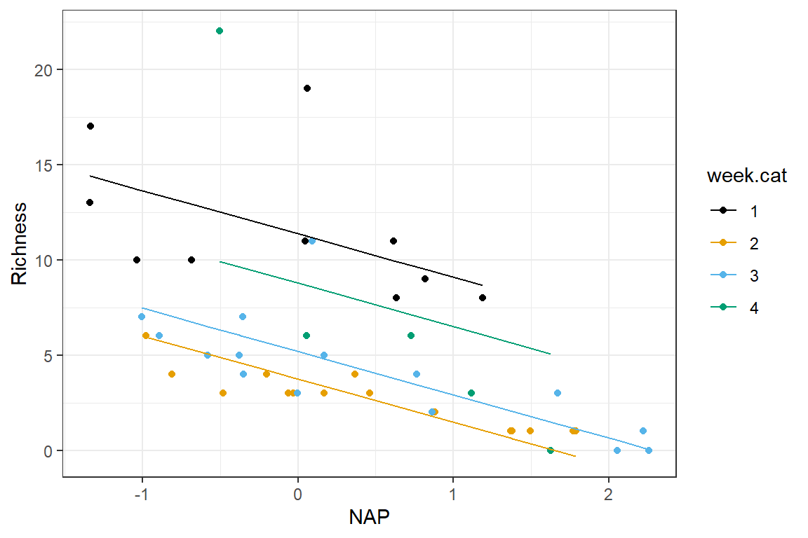
FIGURE 3.5: Expected Richness as a function of NAP for each week in a model without interactions.
This plot makes it clear that the effect of NAP is assumed to be constant for all of the weeks and that the expected Richess when NAP = 0 varies by week (i.e., we have a model with constant slope but varying intercepts).
3.6.2 Means coding
We can fit the same model using means coding by removing the intercept:
##
## Call:
## lm(formula = Richness ~ NAP + week.cat - 1, data = RIKZdat)
##
## Residuals:
##     Min      1Q  Median      3Q     Max
## -5.0788 -1.4014 -0.3633  0.6500 12.0845
##
## Coefficients:
##           Estimate Std. Error t value Pr(>|t|)
## NAP        -2.2708     0.4678  -4.854 1.88e-05 ***
## week.cat1  11.3677     0.9459  12.017 7.48e-15 ***
## week.cat2   3.7426     0.8026   4.663 3.44e-05 ***
## week.cat3   5.1897     0.7979   6.505 9.24e-08 ***
## week.cat4   8.7734     1.3657   6.424 1.20e-07 ***
## ---
## Signif. codes:  0 '***' 0.001 '**' 0.01 '*' 0.05 '.' 0.1 ' ' 1
##
## Residual standard error: 2.987 on 40 degrees of freedom
## Multiple R-squared:  0.8604, Adjusted R-squared:  0.843
## F-statistic: 49.32 on 5 and 40 DF,  p-value: 4.676e-16
We see that the coefficient for week.cat1 is identical to the intercept in the effects model, since week 1 is the reference level in that model. In addition, the other coefficients for the week.cat variables represent the intercepts in the other weeks. If we look at the design matrix for our same 4 observations, we see R creates a separate dummy variable for each week and that the intercept column has been removed.
##       NAP week.cat1 week.cat2 week.cat3 week.cat4
## 10 -1.334         1         0         0         0
## 20 -0.811         0         1         0         0
## 30  0.766         0         0         1         0
## 25  0.054         0         0         0         1
Thus, the means model is parameterized with a separate intercept for each week and can be written as:
\[\begin{equation*} \begin{bmatrix}17 \\ 4 \\ 4 \\ 6 \end{bmatrix} = \begin{bmatrix} -1.134 & 1 & 0 & 0 & 0 \\ -0.811 & 0 & 1 & 0 & 0 \\ 0.766 & 0 & 0 & 1 & 0 \\ 0.054 & 0 & 0 & 0 & 1 \end{bmatrix} \times \begin{bmatrix} \beta_1 \\ \beta_2 \\ \beta_3 \\ \beta_4 \\ \beta_5 \end{bmatrix} + \begin{bmatrix} \epsilon_1 \\ \epsilon_2 \\ \epsilon_3 \\ \epsilon_4 \\ \end{bmatrix} \end{equation*}\]
3.7 Models with interactions
Let’s inspect the residuals from our model fit with effects coding for week.cat plus NAP (the residuals will be identical using either model formulation, though). In this case, we will see how we can create our own customized residual plot using the fortify function along with ggplot (the fortify function in the broom package augments the data set used to fit the model with various outputs from the fitted model, including fitted values and residuals).
  Richness    NAP week.cat      .hat   .sigma      .cooksd   .fitted     .resid
1       11  0.045        1 0.1005319 3.025215 0.0001963069 11.265517 -0.2655173
2       10 -1.036        1 0.1213725 2.958047 0.0487598818 13.720207 -3.7202072
3       13 -1.336        1 0.1373130 3.015884 0.0081202327 14.401435 -1.4014348
4       11  0.616        1 0.1126489 3.020466 0.0034083423  9.968914  1.0310858
5       10 -0.684        1 0.1082954 2.984729 0.0260386947 12.920900 -2.9209002
6        8  1.190        1 0.1409419 3.023361 0.0018954268  8.665499 -0.6654988
    .stdresid
1 -0.09371168
2 -1.32849079
3 -0.50505662
4  0.36638770
5 -1.03538063
6 -0.24034207ggplot(fortify(lm.ancova)) + geom_point(aes(x = .fitted, y = .resid, col = week.cat)) +
geom_hline(yintercept = 0)+theme_bw() + scale_colour_colorblind()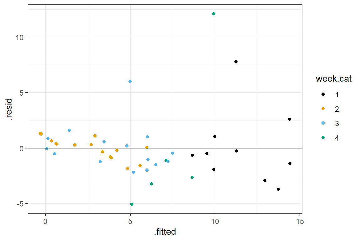
FIGURE 3.6: Residual versus fitted value plot, ANCOVA model
This plot seems to suggest that the residuals increase in variance with higher fitted values (this is common when modeling count data16). There are also a few really residuals with really high absolute values.
Think-pair-share: How can we address these issues?
It is not uncommon to find that model assumptions are not met perfectly when analyzing real data. When this happens, it is tempting to search for model-based solutions, which can send you down a spiraling path towards models with more and more complexity, landing you well outside your comfort zone. We will discuss these challenges more down the road when we cover modeling strategies (see Section 8). For now, let’s assume a colleague of yours tries to improve the fit of your model by adding an interaction between NAP and week.cat.17
3.7.1 Effects coding
We can include an interaction between NAP and week.cat in R using either Richness ~ NAP * week.cat or Richness ~NAP + week.cat + NAP:week.cat:
Call:
lm(formula = Richness ~ NAP * week.cat, data = RIKZdat)

Residuals:
    Min      1Q  Median      3Q     Max
-6.3022 -0.9442 -0.2946  0.3383  7.7103

Coefficients:
              Estimate Std. Error t value Pr(>|t|)
(Intercept)   11.40561    0.77730  14.673  < 2e-16 ***
NAP           -1.90016    0.87000  -2.184 0.035369 *
week.cat2     -8.04029    1.05519  -7.620 4.30e-09 ***
week.cat3     -6.37154    1.03168  -6.176 3.63e-07 ***
week.cat4      1.37721    1.60036   0.861 0.395020
NAP:week.cat2  0.42558    1.12008   0.380 0.706152
NAP:week.cat3 -0.01344    1.04246  -0.013 0.989782
NAP:week.cat4 -7.00002    1.68721  -4.149 0.000188 ***
---
Signif. codes:  0 '***' 0.001 '**' 0.01 '*' 0.05 '.' 0.1 ' ' 1

Residual standard error: 2.442 on 37 degrees of freedom
Multiple R-squared:  0.7997,    Adjusted R-squared:  0.7618
F-statistic: 21.11 on 7 and 37 DF,  p-value: 3.935e-11
Let’s look again at the model matrix to help us write out and understand the model:
##    Richness week    NAP
## 10       17    1 -1.334
## 20        4    2 -0.811
## 30        4    3  0.766
## 25 6 4 0.054## (Intercept) NAP week.cat2 week.cat3 week.cat4 NAP:week.cat2 NAP:week.cat3
## 10 1 -1.334 0 0 0 0.000 0.000
## 20 1 -0.811 1 0 0 -0.811 0.000
## 30 1 0.766 0 1 0 0.000 0.766
## 25 1 0.054 0 0 1 0.000 0.000
## NAP:week.cat4
## 10 0.000
## 20 0.000
## 30 0.000
## 25 0.054Here, we see that we added 3 new predictors to our design matrix last seen in Section 3.6. These columns are formed by multiplying our original 3 dummy variables (indicating weeks 2, 3, and 4) by NAP. Thus, our model can be written as:
\[\begin{gather} Richness_i = \beta_0 + \beta_1NAP_i + \beta_2I(week = 2)_i + \beta_3I(week = 3)_i + \beta_4I(week = 4)_i + \nonumber \\ \beta_5NAP_iI(week = 2)_i + \beta_6NAP_iI(week = 3)_i + \beta_7NAP_iI(week = 4)_i + \epsilon_i \nonumber \end{gather}\]
Or, in matrix notation (for our 4 observations above:
\[\begin{equation*} \begin{bmatrix}11 \\ 10 \\ 13 \\ 11 \\ \end{bmatrix} = \begin{bmatrix}1 & -1.334 & 0 & 0 & 0 & 0 & 0 & 0 \\ 1 & -0.811 & 1 & 0 & 0 & -0.811 & 0 & 0\\ 1 & 0.766 & 0 & 1 & 0 & 0 & 0.766 & 0 \\ 1 & 0.054 & 0 & 0 & 1 & 0 & 0 & 0.054 \end{bmatrix} \times \begin{bmatrix} \beta_0 \\ \beta_1 \\ \beta_2 \\ \beta_3 \\ \beta_4 \\ \beta_5 \\ \beta_6 \\ \beta_7 \end{bmatrix} + \begin{bmatrix} \epsilon_1 \\ \epsilon_2 \\ \epsilon_3 \\ \epsilon_4 \\ \end{bmatrix} \end{equation*}\]
In this model, we have a separate slope and intercept for each week, which becomes more evident when we write out equations for each week in which we collect like terms:
- Week 1: \(Richness_i = \beta_0 + \beta_1NAP_i + \epsilon_i\)
- Week 2: \(Richness_i = [\beta_0 + \beta_2(1)] + [\beta_1 + \beta_5(1)]NAP_i + \epsilon_i\)
- Week 3: \(Richness_i = [\beta_0 + \beta_3(1)] + [\beta_1 + \beta_6(1)]NAP_i + \epsilon_i\)
- Week 4: \(Richness_i = [\beta_0 + \beta_4(1)] + [\beta_1 + \beta_7(1)]NAP_i + \epsilon_i\)
Thus, we see that \(\beta_0\) and \(\beta_1\) represent the intercept and slope for our reference category (week 1). The parameters \(\beta_2\), \(\beta_3\), and \(\beta_4\) represent differences in intercepts for weeks 2, 3, and 4 relative to week 1. And, the parameters \(\beta_5\), \(\beta_6\), and \(\beta_7\) represent differences in slopes (associated with NAP) for weeks 2, 3, and 4 relative to week 1.
We visualize this model below, which highlights that the slope for NAP during week 4 differs from those of the other weeks:
ggplot(fortify(lmfit.inter), aes(NAP, Richness, col = week.cat))+
  geom_line(aes(NAP, .fitted, col = week.cat)) + geom_point() +
  scale_colour_colorblind()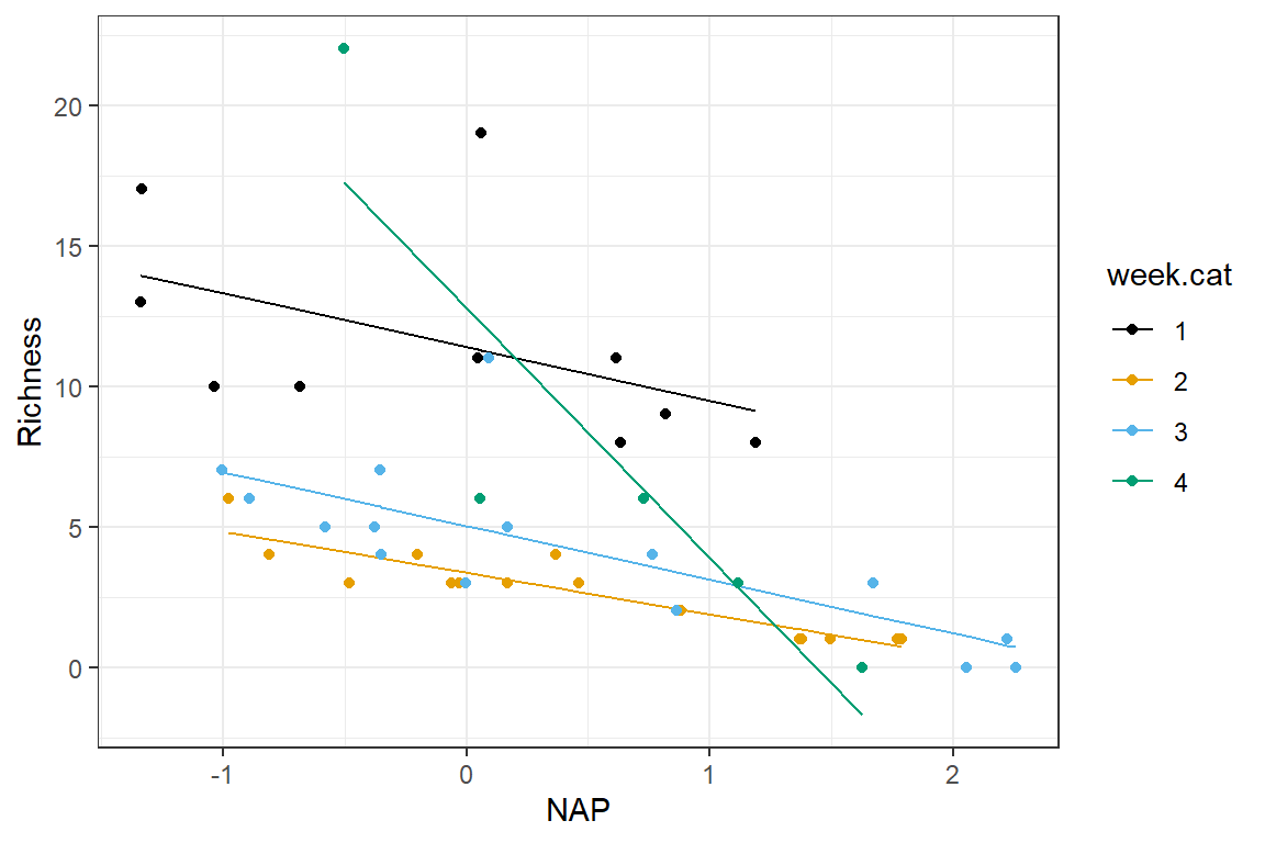
FIGURE 3.7: Regression model with an interaction between NAP and week
3.7.2 Means model
To fit the means parameterization of the model, we need to drop the columns of the design matrix associated with the intercept and slope for week 1 using the following syntax:
##
## Call:
## lm(formula = Richness ~ NAP * week.cat - 1 - NAP, data = RIKZdat)
##
## Residuals:
##     Min      1Q  Median      3Q     Max
## -6.3022 -0.9442 -0.2946  0.3383  7.7103
##
## Coefficients:
##               Estimate Std. Error t value Pr(>|t|)
## week.cat1      11.4056     0.7773  14.673  < 2e-16 ***
## week.cat2       3.3653     0.7136   4.716 3.38e-05 ***
## week.cat3       5.0341     0.6784   7.421 7.85e-09 ***
## week.cat4      12.7828     1.3989   9.138 5.05e-11 ***
## NAP:week.cat1  -1.9002     0.8700  -2.184  0.03537 *
## NAP:week.cat2  -1.4746     0.7055  -2.090  0.04353 *
## NAP:week.cat3  -1.9136     0.5743  -3.332  0.00197 **
## NAP:week.cat4  -8.9002     1.4456  -6.157 3.85e-07 ***
## ---
## Signif. codes:  0 '***' 0.001 '**' 0.01 '*' 0.05 '.' 0.1 ' ' 1
##
## Residual standard error: 2.442 on 37 degrees of freedom
## Multiple R-squared:  0.9138, Adjusted R-squared:  0.8951
## F-statistic:    49 on 8 and 37 DF,  p-value: < 2.2e-16
We can inspect the design matrix and write the model for our 4 observations in matrix notation:
\[\begin{equation*} \begin{bmatrix}11 \\ 10 \\ 13 \\ 11 \\ \end{bmatrix} = \begin{bmatrix}1 & 0 & 0 & 0 & -1.334 & 0 & 0 & 0 \\ 0 & 1 & 0 & 0 & 0 & -0.811 & 0 & 0\\ 0 & 0 & 1 & 0 & 0 & 0 & 0.766 & 0 \\ 0 & 0 & 0 & 1 & 0 & 0 & 0 & 0.054 \end{bmatrix} \times \begin{bmatrix} \beta_1 \\ \beta_2 \\ \beta_3 \\ \beta_4 \\ \beta_5 \\ \beta_6 \\ \beta_7 \\ \beta_8 \end{bmatrix} + \begin{bmatrix} \epsilon_1 \\ \epsilon_2 \\ \epsilon_3 \\ \epsilon_4 \\ \end{bmatrix} \end{equation*}\]
##    week.cat1 week.cat2 week.cat3 week.cat4 NAP:week.cat1 NAP:week.cat2
## 10         1         0         0         0        -1.334         0.000
## 20         0         1         0         0         0.000        -0.811
## 30         0         0         1         0         0.000         0.000
## 25         0         0         0         1         0.000         0.000
##    NAP:week.cat3 NAP:week.cat4
## 10         0.000         0.000
## 20         0.000         0.000
## 30         0.766         0.000
## 25         0.000         0.054
In this formulation of the model, we directly estimate separate intercepts and slopes for each week (rather than parameters that describe deviations from a reference group):
\[\begin{gather} Richness_i = \beta_1I(week=1)_i + \beta_2I(week = 2)_i + \beta_3I(week = 3)_i + \beta_4I(week = 4)_i + \nonumber \\ \beta_5NAP_iI(week=1) +\beta_6NAP_iI(week = 2)_i + \beta_7NAP_iI(week = 3)_i + \beta_8NAP_iI(week = 4)_i + \epsilon_i \nonumber \end{gather}\]
This gives us the following equations for the observations from each week:
- Week 1: \(Richness_i = \beta_1 + \beta_5NAP_i + \epsilon_i\)
- Week 2: \(Richness_i = \beta_2 + \beta_6NAP_i + \epsilon_i\)
- Week 3: \(Richness_i = \beta_3 + \beta_7NAP_i + \epsilon_i\)
- Week 4: \(Richness_i = \beta_4 + \beta_8NAP_i + \epsilon_i\)
3.7.3 Creating flexible models with dummy variables
After looking at Figure (3.7), we might decide that we want to fit a model that allows each week to have its own intercept, but that the effect of NAP is the same in weeks 1-3 and differs only in week 4. If we understand how categorical variables are encoded in regression models, we can fit this model quite easily. We need to include week.cat to allow each week to have its own intercept. We also create a single dummy variable (equal to 1 if week is equal to 4 and 0 otherwise) and include the interaction of this dummy variable with NAP:
lm.datadriven <- lm(Richness ~ NAP + week.cat + NAP:I(week==4), data = RIKZdat)
summary(lm.datadriven)
##
## Call:
## lm(formula = Richness ~ NAP + week.cat + NAP:I(week == 4), data = RIKZdat)
##
## Residuals:
## Min 1Q Median 3Q Max
## -6.3022 -0.9762 -0.0838 0.6269 7.6894
##
## Coefficients:
## Estimate Std. Error t value Pr(>|t|)
## (Intercept) 11.4187 0.7558 15.108 < 2e-16 ***
## NAP -1.7722 0.3875 -4.573 4.77e-05 ***
## week.cat2 -7.9124 0.9996 -7.915 1.23e-09 ***
## week.cat3 -6.4463 0.9965 -6.469 1.16e-07 ***
## week.cat4 1.3641 1.5623 0.873 0.388
## NAP:I(week == 4)TRUE -7.1280 1.4652 -4.865 1.92e-05 ***
## ---
## Signif. codes: 0 '***' 0.001 '**' 0.01 '*' 0.05 '.' 0.1 ' ' 1
##
## Residual standard error: 2.387 on 39 degrees of freedom
## Multiple R-squared: 0.7983, Adjusted R-squared: 0.7725
## F-statistic: 30.88 on 5 and 39 DF, p-value: 1.425e-12We can write down this model as:
\[\begin{gather} Richness_i = \beta_0 + \beta_1NAP_i + \beta_2I(week = 2)_i + \beta_3I(week = 3)_i + \beta_4I(week = 4)_i + \nonumber \\ \beta_5NAP_iI(week = 4)_i + \epsilon_i \nonumber \end{gather}\]
Which implies:
- Week 1: \(Richness_i = \beta_0 + \beta_1NAP_i + \epsilon_i\)
- Week 2: \(Richness_i = [\beta_0 + \beta_2] + \beta_1NAP_i + \epsilon_i\)
- Week 3: \(Richness_i = [\beta_0 + \beta_3] + \beta_1NAP_i + \epsilon_i\)
- Week 4: \(Richness_i = [\beta_0 + \beta_4] + [\beta_1 + \beta_5]NAP_i + \epsilon_i\)
Let’s plot the fitted model of the expected Richness as a function of NAP for each week:
ggplot(fortify(lm.datadriven), aes(NAP, Richness, col = week.cat))+
  geom_line(aes(NAP, .fitted, col = week.cat)) + geom_point() +
  scale_colour_colorblind()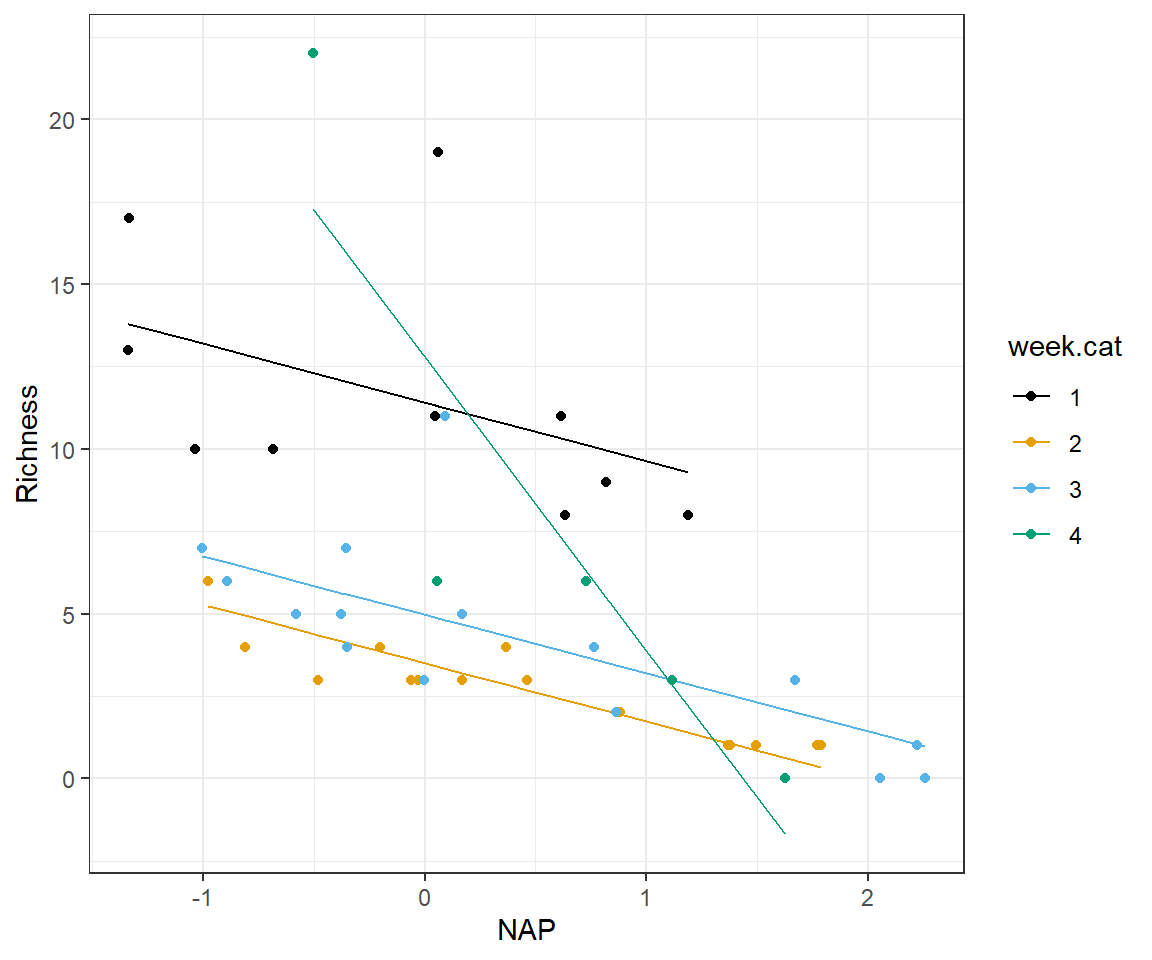
FIGURE 3.8: Species richness versus NAP for a model allowing the effect of NAP to differ in week 4 versus all other weeks.
Although these results may look convincing, we arrived at this result in a very data-driven way. As we will discuss in Section 8, it is easy to develop models that fit your data well but that perform poorly when applied to new data. In general, you should be skeptical of relationships discovered based on intensive data exploration that were not expected a priori. Also, remember that this is an unbalanced design, with only 5 observations during week 4. Hence, this interaction model should be interpreted with great caution. It is quite possible that we are just fitting a model that explains noise in the data. Note, for example, the outlier present in the data from week 4. this point could be the result of measurement error or some other factor that we have not accounted for in our model and the sole reasons for the “need” for the interaction. In addition, if we plot residuals versus fitted values, we still see there are several large outliers in our residuals. So issues remain with our model that warrant further consideration.
ggplot(fortify(lm.datadriven), aes(.fitted, .resid, col = week.cat))+
  geom_point() + geom_hline(yintercept = 0) +
  scale_colour_colorblind()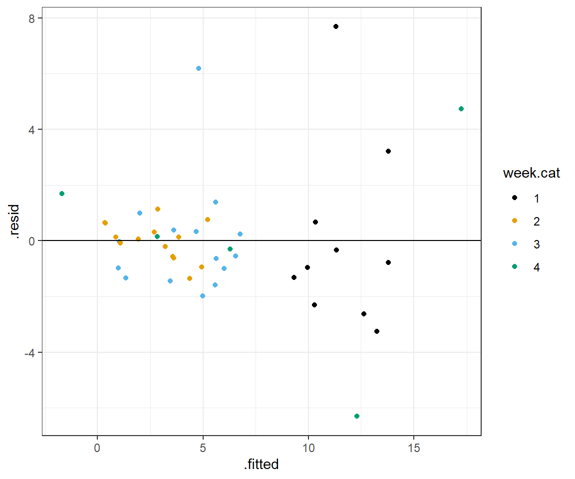
FIGURE 3.9: Residual versus fitted value plot for the model allowing the effect of NAP to differ in week 4 versus all other weeks.
3.7.4 Improving parameter interpretation through centering
When we fit a model with an interaction between a continuous and categorical variable, we are explicitly assuming that the difference between any 2 groups depends on the value of the continuous variable – for example, the difference in species richness between weeks 1 and 2 depends on the value of NAP (Figure 3.7). Further, the coefficients associated with the categorical variable represent differences in intercepts, or in other words, mean responses when all other variables are set to 0. As we saw in Section 1.2, intercepts may be difficult to interpret or misleading when they require extrapolating outside of the range of the observed data.
Centering the continuous variable can make it easier to interpret the parameters associated with the categorical variable in models with interactions (Schielzeth, 2010). For example, if we refit our model after centering NAP by its mean, then the intercepts will represent contrasts between each group and the reference group when NAP is set to its mean (rather than 0) if we use effects coding, or differences between the groups when NAP is set to its mean value and we use means coding.
3.8 Pairwise comparisons
Consider the model below, fit to the RIKZ data set. The model includes two quantitative variables (NAP and exposure) and a categorical variable with more than 2 categories (week).
Call:
lm(formula = Richness ~ NAP + exposure + week.cat, data = RIKZdat)

Residuals:
   Min     1Q Median     3Q    Max
-4.912 -1.621 -0.313  1.004 11.903

Coefficients:
            Estimate Std. Error t value Pr(>|t|)
(Intercept)  23.9262     7.3960   3.235  0.00248 **
NAP          -2.4344     0.4668  -5.215 6.33e-06 ***
exposure     -1.3972     0.8164  -1.711  0.09495 .
week.cat2    -4.7364     2.0827  -2.274  0.02854 *
week.cat3    -4.2269     1.6671  -2.535  0.01535 *
week.cat4    -1.0814     1.8548  -0.583  0.56323
---
Signif. codes:  0 '***' 0.001 '**' 0.01 '*' 0.05 '.' 0.1 ' ' 1

Residual standard error: 2.918 on 39 degrees of freedom
Multiple R-squared:  0.6986,    Adjusted R-squared:  0.6599
F-statistic: 18.08 on 5 and 39 DF,  p-value: 2.991e-09
For NAP and exposure, we can use the t-tests in the output above to test whether there is sufficient evidence to conclude the coefficients are not equal to 0. We can also see in the output whether we have evidence to suggest there are differences between week 2 and week 1, week 3 and week 1, and week 4 and week 1. What if we want to test for differences between say weeks 2 and 4, or between all pairs of weeks we have?
This question brings up the thorny issue of multiple comparisons. There are “4 choose 2” = 6 possible pairwise comparisons we could consider when comparing the 4 weeks, and in general \({k \choose 2} = \frac{k!}{2!(k-2)!}\) possible comparisons if there are \(k\) groups. If the probability of making a type I error (i.e., rejecting the null hypothesis when it is true) is \(\alpha\), and each test is independent from all the other tests, then we would have a \(1- (1-\alpha)^{n_{tests}}\) (roughly an 26% chance if \(\alpha = 0.05\) and we conduct 6 tests) of rejecting at least one null hypothesis even if all of them were true; this error rate is often referred to as the family-wise error rate. The problem increases with the number of categories associated with the categorical variable and applies also to confidence intervals (i.e., the chance of at least one confidence interval failing to capture the true mean pairwise difference increases with the number of confidence intervals considered).
The usual way of dealing with multiple comparisons is to apply a correction factor that adjusts the p-values associated with individual hypothesis tests (or, alternatively, adjusts the critical values with which the p-values are compared when deciding if there is evidence to reject the null hypothesis). Similarly, one can make adjustments to confidence intervals to make them wider in hopes of controlling the family-wise error rate. There are multiple packages in R for conducting pairwise comparisons with adjustments. We briefly demonstrate one option using the emmeans package (Lenth, 2021). We begin by estimating the mean Richness for each week when NAP and exposure are set to their mean values using the enmeans function:
##  week.cat emmean    SE df lower.CL upper.CL
##  1          8.80 1.406 39     5.95    11.64
##  2          4.06 0.995 39     2.05     6.07
##  3          4.57 0.761 39     3.03     6.11
##  4          7.72 1.320 39     5.05    10.38
##
## Confidence level used: 0.95
We can then use the pairs function to calculate all 6 pairwise differences between weekly means and test whether these differences are statistically significant (i.e., whether we have evidence that the true difference is likely non-zero). We can also request confidence intervals for the pairwise differences in means by supplying the argument infer = c(TRUE, TRUE).
##  contrast estimate   SE df lower.CL upper.CL t.ratio p.value
##  1 - 2       4.736 2.08 39   -0.852   10.325   2.274  0.1217
##  1 - 3       4.227 1.67 39   -0.247    8.700   2.535  0.0699
##  1 - 4       1.081 1.85 39   -3.896    6.058   0.583  0.9366
##  2 - 3      -0.509 1.20 39   -3.725    2.706  -0.425  0.9738
##  2 - 4      -3.655 1.71 39   -8.241    0.931  -2.139  0.1589
##  3 - 4      -3.146 1.53 39   -7.252    0.961  -2.055  0.1858
##
## Confidence level used: 0.95
## Conf-level adjustment: tukey method for comparing a family of 4 estimates
## P value adjustment: tukey method for comparing a family of 4 estimates
Each row represents a different pairwise comparison identified by the label in the first column. By default, emmeans uses Tukey’s Honest Significant Difference (HSD) to adjust the p-values and confidence intervals associated with each comparison (Abdi & Williams, 2010), thus controlling the family-wise error rate (i.e., the probability that we incorrectly reject at least 1 null hypothesis when all of the null hypotheses are true). Using a family-wise error rate of \(\alpha = 0.05\), we would conclude that we do not have enough evidence to reject the null hypothesis for any of the pairwise comparisons, as they all have p-values > 0.05. We can see our conclusions are more conservative than if we had not done any adjustments:
##  contrast estimate   SE df lower.CL upper.CL t.ratio p.value
##  1 - 2       4.736 2.08 39    0.524    8.949   2.274  0.0285
##  1 - 3       4.227 1.67 39    0.855    7.599   2.535  0.0153
##  1 - 4       1.081 1.85 39   -2.670    4.833   0.583  0.5632
##  2 - 3      -0.509 1.20 39   -2.933    1.914  -0.425  0.6730
##  2 - 4      -3.655 1.71 39   -7.112   -0.198  -2.139  0.0388
##  3 - 4      -3.146 1.53 39   -6.241   -0.050  -2.055  0.0466
##
## Confidence level used: 0.95
Without any adjustment, we would have concluded that weeks 1 and 2, weeks 1 and 3, weeks 2 and 4, and weeks 3 and 4 all differ from one another. Clearly, then, there is a tradeoff involved when adjusting for multiple comparisons. We can reduce the family-wise type I error rate at the expense of increasing the type II error rate (failing to reject a null hypotheses when it is indeed false). Thus, correcting for multiple comparisons is not without its critics (e.g., Perneger, 1998; Moran, 2003; Nakagawa, 2004). Rather than attempt to control the family-wise error rate (i.e., probability of incorrectly rejecting one or more null hypotheses), many statisticians now advocate for controlling the false discovery rate, defined as the proportion of significant results that reflect type I errors (see e.g., Benjamini & Hochberg, 1995; García, 2004; Verhoeven, Simonsen, & McIntyre, 2005; Pike, 2011). In other words, rather than attempt to avoid rejecting any null hypotheses that are true, the goal is to ensure that most of the hypotheses that are rejected are indeed false. Controlling the false discovery rate results in more powerful tests, meaning we are more likely to reject hypotheses when they are false, and less conservative adjustments than controlling for the family-wise error rate.
Another option that is sometimes used to control the family-wise error rate is what is called Fisher’s least significant difference (LSD) procedure in which a global, multiple degree-of-freedom test is conducted first. If this test is significant, then one proceeds with further pairwise comparisons. If the global test is not significant, then no pairwise comparisons are conducted. This approach is capable of controlling the family-wise error rate when there are only 3 groups under consideration (Meier, 2006). We discuss the multiple degree-of-freedom test in Section 3.9. Lastly, it is often beneficial to limit the number of tests conducted to just those comparisons that are of primary interest.
3.9 Multiple degree-of-freedom hypothesis tests
The Fisher’s LSD procedure would require us to first test the global null hypothesis that the coefficients for week.cat2, week.cat3 and week.cat4 are all 0 (i.e., all weeks have the same species Richness after adjusting for NAP and exposure) versus an alternative hypothesis that at least 1 of the coefficients is non-zero. Tests of joint hypotheses (i.e., hypotheses involving multiple parameters set to different values, usually 0), can be conducted using either a \(\chi^2\) or \(F\) distribution. Tests using the \(\chi^2\) distribution are usually based on large sample approximations that lead to a Normal distribution (the square of a Normal random variable is distributed as \(\chi^2_1\)). The \(F\) distribution, like the \(t-\)distribution, is more appropriate when all of the assumptions of the linear regression model are met. The two tests will be equivalent as sample sizes approach infinity. The \(\chi^2\) and \(F\) distributions only assign probabilities to positive values and therefore, p-values are calculated as areas to the right of our test statistic, calculated from the observed data.
F-statistics have an associated numerator and denominator degrees of freedom and can be most easily understood in terms of comparing two models – a full model (\(M_F\)) and a reduced model (\(M_R\)) in which some subset of parameters have been set equal to 0. Let \(p_F\) and \(p_R\) be the number of parameters in the full and reduced models, respectively. The numerator degrees of freedom, \(k_1\), is equal to the difference in the number of parameters (\(k_1 = p_F - p_R = 3\) when testing the null hypothesis that the coefficients for week.cat2, week.cat3 and week.cat4 are all 0). The denominator degrees of freedom, \(k_2\), is determined from the full model that includes these additional parameters and is equal to \(n-p_F\) where \(n\) is the sample size. The \(F-\)statistic can be calculated as:
\[\begin{gather} F = \frac{(SSE_{M_R}- SSE_{M_F})/(p_F- p_R)}{SSE_{M_F}/(n-p_F)} = \frac{(SSR_{M_F}- SSR_{M_R})/(p_F- p_R)}{SSE_{M_F}/(n-p_F)}, \tag{3.1} \end{gather}\]
where \(SSE_{M_R}\) and \(SSR_{M_R}\) are the residual and regression sums-of-squares for the restricted/constrained model (in this case, with parameters for week.cat2, week.cat3, and week.cat4 set to 0), and \(SSE_{M_F}\) and \(SSR_{M_F}\) are the residual and regression sums-of-squares for the full model (where these parameters are also estimated). Thus, the numerator captures the additional variability that is explained by including the additional parameters and should be close to 0 if the null hypothesis is true.
When using software to calculate sums of squares, you may be surprised to learn that sums-of-squares may be calculated in different ways, depending on whether we consider constructing a model sequentially, adding one variable at a time (so called type I sums of squares), or we consider removing a variable from the model containing all predictors (type III sums of squares)18. I.e., whether we build the model in a “forward” or “backward” direction influences what other variables are included or adjusted for when calculating regression sums of squares. When testing hypotheses, I recommend a backwards model-selection approach, which is implemented using the Anova function in the car package. By contrast, the anova function in base R will implement a sequential approach, in which case the results of the test will depend on the ordering of the variables when you specify the model.
Let’s start with the Anova function:
Anova Table (Type II tests)

Response: Richness
          Sum Sq Df F value    Pr(>F)
NAP       231.59  1 27.1999 6.335e-06 ***
exposure   24.94  1  2.9289   0.09495 .
week.cat   73.19  3  2.8654   0.04888 *
Residuals 332.07 39
---
Signif. codes:  0 '***' 0.001 '**' 0.01 '*' 0.05 '.' 0.1 ' ' 1
The Anova function returns tests appropriate for backwards selection (see Section 8.3.1) - meaning that these tests determine if we have enough evidence to suggest that the variable of interest is associated with the response variable, after adjusting for the other variables in the model. In this case, both the full and reduced models include all other variables. The F-tests here for NAP and exposure are equivalent to the t-tests in the summary of the lm (in fact, the F-statistics are equal to the square of the \(t-\)statistics we saw previously). The advantage of using Anova is that it also returns a multiple degree-of-freedom test for week.cat. The associated p-value (0.0488) suggests we have enough evidence in the data to conclude that at least one of the weeks differs from the others (in terms of species richness after adjusting for exposure and NAP).
If we had used the anova function, we would end up with a different set of tests resulting from sequentially adding variables one at a time. In this case, the order in which the predictor variables appear matters. We will compare two different calls to lm below to demonstrate this:
Analysis of Variance Table

Response: Richness
          Df Sum Sq Mean Sq F value    Pr(>F)
week.cat   3 534.31 178.104 20.9177 3.060e-08 ***
exposure   1   3.67   3.675  0.4316    0.5151
NAP        1 231.59 231.593 27.1999 6.335e-06 ***
Residuals 39 332.07   8.514
---
Signif. codes:  0 '***' 0.001 '**' 0.01 '*' 0.05 '.' 0.1 ' ' 1
The p-values here test whether :
- at least one coefficient associated with
week.catis non-zero in a model that only includesweek.cat(since it was specified first) - the coefficient for
exposureis non-zero in a model withweek.catandexposure - the coefficient for
NAPis non-zero in a model that containsweek.cat,exposure, andNAP.
If we reverse the order variables are entered into the model, we get a different set of p-values, with the test for week.cat now matching the test from the Anova function.
## Analysis of Variance Table
##
## Response: Richness
##           Df Sum Sq Mean Sq F value    Pr(>F)
## NAP        1 357.53  357.53 41.9907 1.117e-07 ***
## exposure   1 338.86  338.86 39.7977 1.931e-07 ***
## week.cat   3  73.19   24.40  2.8654   0.04888 *
## Residuals 39 332.07    8.51
## ---
## Signif. codes:  0 '***' 0.001 '**' 0.01 '*' 0.05 '.' 0.1 ' ' 1
In addition to using an \(F-\)test for categorical variables with more than 2-levels, we can also use an \(F-\)test to evaluate whether any of our predictors explain a significant proportion of variability in the response as we will see in the next section.
3.10 Regression F-statistic
When using the summary function with a fitted regression model, you may notice an F-statistic and p-value at the bottom of the output:
##
## Call:
## lm(formula = Richness ~ NAP + exposure + week.cat, data = RIKZdat)
##
## Residuals:
##    Min     1Q Median     3Q    Max
## -4.912 -1.621 -0.313  1.004 11.903
##
## Coefficients:
##             Estimate Std. Error t value Pr(>|t|)
## (Intercept)  23.9262     7.3960   3.235  0.00248 **
## NAP          -2.4344     0.4668  -5.215 6.33e-06 ***
## exposure     -1.3972     0.8164  -1.711  0.09495 .
## week.cat2    -4.7364     2.0827  -2.274  0.02854 *
## week.cat3    -4.2269     1.6671  -2.535  0.01535 *
## week.cat4    -1.0814     1.8548  -0.583  0.56323
## ---
## Signif. codes:  0 '***' 0.001 '**' 0.01 '*' 0.05 '.' 0.1 ' ' 1
##
## Residual standard error: 2.918 on 39 degrees of freedom
## Multiple R-squared:  0.6986, Adjusted R-squared:  0.6599
## F-statistic: 18.08 on 5 and 39 DF,  p-value: 2.991e-09
This F-statistic is testing whether all regression coefficients (other than the intercept) are simultaneously 0 versus an alternative hypothesis that at least one of the coefficients is non-zero. Thus, the numerator degrees of freedom is equal to \(p-1\) where \(p\) is the number of parameters in the model (\(p-1 = 5\) in the above case). The denominator degrees of freedom is again equal to \(n-p\). Similar to the idea behind Fisher’s least significant difference (LSD) procedure, we might consider only testing hypotheses involving individual coefficients when this global test is rejected as one way to reduce the family-wise type I error rate.
3.11 Contrasts: Estimation of linear combinations of parameters
Often, we are interested in estimating some linear combination (i.e., a weighted sum) of our regression parameters. Consider again the model with only NAP and week.cat fit using effects coding:
\[\begin{equation*} Richness_i = \beta_0 + \beta_1NAP_i + \beta_2I(week = 2)_i + \beta_3I(week=3)_i + \beta_4I(week=4)_i + \epsilon_i, \end{equation*}\]
We saw how we can use the functions in the emmeans package to estimate the difference in Richness between weeks 2 and 3 (as well as between other weeks), while controlling for NAP. We can estimate this contrast between mean Richness in weeks 2 and 3 as: \(\hat{\beta}_2 - \hat{\beta}_3\). To correctly estimate its uncertainty requires considering how much \(\hat{\beta_2}\) and \(\hat{\beta}_3\) vary as well as how much they co-vary across data sets if we could replicate the sampling design many times. I.e., we must consider the variance/covariance matrix of our regression parameter estimators, \(\hat{\Sigma}_{\hat{\beta}}\):
\[\hat{\Sigma}_{\hat{\beta}}= \begin{bmatrix} var(\hat{\beta}_0) & cov(\hat{\beta}_0, \hat{\beta_1}) & cov(\hat{\beta}_0, \hat{\beta_2}) & cov(\hat{\beta}_0, \hat{\beta_3}) & cov(\hat{\beta}_0, \hat{\beta_4})\\ cov(\hat{\beta}_0, \hat{\beta_1}) & var(\hat{\beta}_1) & cov(\hat{\beta}_1, \hat{\beta_2}) & cov(\hat{\beta}_1, \hat{\beta_3}) & cov(\hat{\beta}_1, \hat{\beta_4}) \\ cov(\hat{\beta}_0, \hat{\beta_2}) & cov(\hat{\beta}_1, \hat{\beta_2}) & var(\hat{\beta}_2) & cov(\hat{\beta}_2, \hat{\beta_3}) & cov(\hat{\beta}_2, \hat{\beta_4})\\ cov(\hat{\beta}_0, \hat{\beta_3}) & cov(\hat{\beta}_1, \hat{\beta_3}) & cov(\hat{\beta}_2, \hat{\beta_3}) & var(\hat{\beta}_3) & cov(\hat{\beta}_3, \hat{\beta_4})\\ cov(\hat{\beta}_0, \hat{\beta_4}) & cov(\hat{\beta}_1, \hat{\beta_4}) & cov(\hat{\beta}_2, \hat{\beta_4}) & cov(\hat{\beta}_3, \hat{\beta_4}) & var(\hat{\beta}_4) \end{bmatrix}\].
For constants \(a\) and \(b\), the \(var(ax + by) = a^2var(x) + b^2var(y)+ 2abcov(x,y)\). Thus, \(var(\hat{\beta}_2 - \hat{\beta}_3) = var(\hat{\beta}_2) + var(\hat{\beta}_3) + 2cov(\hat{\beta}_2, \hat{\beta_3})\). We can calculate this variance using matrix multiplication. Define the transpose of a column vector, \(c\) as \(c' =c(0, 0, 1, -1, 0)\), which we will use to estimate our contrast of interest via matrix multiplication:
\[c'\hat{\beta} = \begin{bmatrix} 0 & 0 & 1 & -1 & 0\end{bmatrix}\begin{bmatrix} \hat{\beta}_0 \\ \hat{\beta}_1 \\ \hat{\beta}_2 \\\hat{\beta}_3 \\ \hat{\beta}_4\end{bmatrix} = \hat{\beta}_2 - \hat{\beta}_3\].
The variance of this contrast is given by:
\[c'\Sigma_b c = \begin{bmatrix} 0 & 0 & 1 & -1 & 0\end{bmatrix}\begin{bmatrix}
var(\hat{\beta}_0) & cov(\hat{\beta}_0, \hat{\beta_1}) & cov(\hat{\beta}_0, \hat{\beta_2}) & cov(\hat{\beta}_0, \hat{\beta_3}) & cov(\hat{\beta}_0, \hat{\beta_4})\\
cov(\hat{\beta}_0, \hat{\beta_1}) & var(\hat{\beta}_1) & cov(\hat{\beta}_1, \hat{\beta_2}) & cov(\hat{\beta}_1, \hat{\beta_3}) & cov(\hat{\beta}_1, \hat{\beta_4}) \\
cov(\hat{\beta}_0, \hat{\beta_2}) & cov(\hat{\beta}_1, \hat{\beta_2}) & var(\hat{\beta}_2) & cov(\hat{\beta}_2, \hat{\beta_3}) & cov(\hat{\beta}_2, \hat{\beta_4})\\
cov(\hat{\beta}_0, \hat{\beta_3}) & cov(\hat{\beta}_1, \hat{\beta_3}) & cov(\hat{\beta}_2, \hat{\beta_3}) & var(\hat{\beta}_3) & cov(\hat{\beta}_3, \hat{\beta_4})\\
cov(\hat{\beta}_0, \hat{\beta_4}) & cov(\hat{\beta}_1, \hat{\beta_4}) & cov(\hat{\beta}_2, \hat{\beta_4}) & cov(\hat{\beta}_3, \hat{\beta_4}) & var(\hat{\beta}_4)
\end{bmatrix} \begin{bmatrix} 0 \\ 0 \\ 1 \\ -1 \\ 0\end{bmatrix}\].
To verify, let’s calculate the standard error of this contrast (equivalent to the square-root of the variance) using matrix multiplication in R, noting that \(\Sigma_b\) can be obtained using the vcov function applied to our linear model object:
Sigma_b<- vcov(lm.ancova)
cmat <- c(0, 0, 1, -1, 0)
cmat%*%coef(lm.ancova) # estimate of week 2 - week 3
## [,1]
## [1,] -1.447196## [,1]
## [1,] 1.091021## contrast estimate SE df t.ratio p.value
## 1 - 2 7.63 1.25 40 6.105 <.0001
## 1 - 3 6.18 1.25 40 4.961 <.0001
## 1 - 4 2.59 1.67 40 1.554 0.1280
## 2 - 3 -1.45 1.09 40 -1.326 0.1922
## 2 - 4 -5.03 1.54 40 -3.258 0.0023
## 3 - 4 -3.58 1.54 40 -2.320 0.0255We see that we get an equivalent SE to the one returned by the pairs function for the difference between weeks 2 and 3. At this point, you might be wondering why you need to know how to calculate contrasts and their uncertainty using matrix algebra if emmeans will do all the hard work for you. Good question! There are times when you may be interested in something other than a simple pairwise difference. For example, we could test whether the last two weeks had higher species richness, on average, than the first two using \(c' = (0, 1/2, 1/2, -1/2, -1/2)\), giving \(\left(\frac{\hat{\beta}_1 + \hat{\beta}_2}{2}\right) - \left(\frac{\hat{\beta}_3 + \hat{\beta}_4}{2}\right)\). A similar approach was used by Iannarilli, Erb, Arnold, & Fieberg (2021) to test for differences in average encounter rates in a camera trap study where sites were randomized to one of two types of lures and one of two types of camera placement strategies. For a more thorough discussion of the importance of contrasts, see Schad, Vasishth, Hohenstein, & Kliegl (2020).
3.12 Aside: Revisiting F-tests and comparing to Wald \(\chi^2\) tests
In Section 3.9, we considered the F-statistic written in terms of sums of squares. We can also formulate F tests using matrix algebra. Similar to the previous section, we will use \(C\) (here as a matrix instead of a vector) to identify one or more linear combinations of our regression parameters. Let’s consider again the model from Section 3.9:
\[\begin{equation*} Richness_i = \beta_0 + \beta_1NAP_i + \beta_2 exposure_i + \beta_3I(week = 2)_i + \beta_4I(week=3)_i + \beta_5I(week=4)_i + \epsilon_i, \end{equation*}\]
Define our contrast matrix, \(C\) as:
\[\begin{gather} C =\begin{bmatrix}0 & 0 & 0 & 1 & 0 & 0 \\ 0 & 0 & 0 & 0 & 1 & 0 \\ 0 & 0 & 0 & 0 & 0 & 1 \end{bmatrix} \end{gather}\]
Using matrix multiplication, \(C \beta\), identifies the parameters involved in our multiple degree of freedom hypothesis test:
\[\begin{gather} C\beta = \begin{bmatrix}0 & 0 & 0 & 1 & 0 & 0 \\ 0 & 0 & 0 & 0 & 1 & 0 \\ 0 & 0 & 0 & 0 & 0 & 1 \end{bmatrix} \begin{bmatrix}\beta_0\\ \beta_1\\ \beta_2\\ \beta_3\\ \beta_4\\ \beta_5\end{bmatrix} = \begin{bmatrix} \beta_3\\ \beta_4\\ \beta_5\end{bmatrix} \end{gather}\]
The F-statistic can be written as:
\[\begin{equation} F = \frac{1}{k_1} (C\hat{\beta})'(C\hat{\Sigma}_{\hat{\beta}}C')^{-1}(C\hat{\beta}) \tag{3.2} \end{equation}\]
where \(\hat{\Sigma}_{\hat{\beta}}\) is once again our estimated variance-covariance matrix associated with \(\hat{\beta}\). We can use matrix algebra to verify the F-statistic from the test calculated using the Anvoa function:
cmat <- matrix(c(0, 0, 0, 1, 0, 0,
                 0, 0, 0, 0, 1, 0,
                 0, 0, 0, 0, 0, 1), byrow=TRUE, ncol=6)
t(cmat%*%coef(lm.RIKZ))%*%solve(cmat%*%vcov(lm.RIKZ)%*%t(cmat))%*%(cmat%*%coef(lm.RIKZ))/3
## [,1]
## [1,] 2.865437## Anova Table (Type II tests)
##
## Response: Richness
## Sum Sq Df F value Pr(>F)
## NAP 231.59 1 27.1999 6.335e-06 ***
## exposure 24.94 1 2.9289 0.09495 .
## week.cat 73.19 3 2.8654 0.04888 *
## Residuals 332.07 39
## ---
## Signif. codes: 0 '***' 0.001 '**' 0.01 '*' 0.05 '.' 0.1 ' ' 1Alternatively, we could consider a \(\chi^2\) test, with the statistic calculated as follows:
\[\begin{equation} \chi^2 = (C\hat{\beta})'(C\hat{\Sigma}_{\hat{\beta}}C')^{-1}(C\hat{\beta}) \tag{3.3} \end{equation}\]
with degrees of freedom equal to the number of rows in \(C\).
chisq<-t(cmat%*%coef(lm.RIKZ))%*%solve(cmat%*%vcov(lm.RIKZ)%*%t(cmat))%*%(cmat%*%coef(lm.RIKZ))
pchisq(chisq, df=3, lower.tail=FALSE)
## [,1]
## [1,] 0.03516874We get a slightly smaller p-value in this case relative to the \(F-\)test, similar to what you would expect if you used a Normal distribution rather than a t-distribution to conduct a hypothesis test with small sample sizes.
The two tests are asymptotically equivalent (i.e., for large sample sizes). The \(\chi^2\) test can be motivated by noting that asymptotically:
\[C\hat{\beta} \sim N(C\beta, C\hat{\Sigma}_{\hat{\beta}}C')\]
Thus, in the 1-dimensional case, the \(\chi^2\) statistic is equivalent to the square of a z-statistic:
\[\left(\frac{C\hat{\beta} -0}{SE(C\hat{\beta})}\right)^2\]
Lastly, we can also test hypotheses in which the regression parameters are set to specific values other than 0 by replacing \(C\) with \(C - \tilde{\beta}\) in equation (3.2) and (3.3), where \(\tilde{\beta}\) represents the values of \(\beta\) under the null hypothesis.
3.13 Visualizing multiple regression models
Consider a regression model with two explanatory variables, \(X_1\) and \(X_2\).
\[Y_i = \beta_0+X_{i,1}\beta_1 + X_{i,2}\beta_2 + \epsilon_i\]
We have already noted that \(\beta_1\) reflects the “effect” of \(X_1\) on \(Y\) after accounting for \(X_2\). Specifically, it describes the expected change in \(Y\) for every 1 unit increase in \(X_1\) while holding \(X_2\) constant. If we want to visualize this effect, a simple strategy that is often used is to:
- Create a data set with \(X_1\) taking on a range of values and with \(X_2\) set to its mean value (for quantitative predictors) or its modal value (for categorical predictors).
- Generate predictions, \(\hat{Y}\), for each value in this data set and plot \(\hat{Y}\) versus \(X_1\).
This strategy is easy to implement using the predict function in R and generalizes to models with more than two predictors. In addition, there are various packages that will construct this type of effect plot for you. In particular, we will look at the effects package (Fox, 2003; Fox & Weisberg, 2018, 2019b) for creating these types plots in Section 16.
When fitting a linear regression model with only 1 predictor, it is common to create a scatterplot of \(Y\) versus \(X\) along with the fitted regression line to visualize the effect of \(X\) on \(Y\). This type of plot allows us to quickly visualize the amount of variability in \(Y\) explained by \(X\) (and also the amount of unexplained variability remaining). It would be nice to have a similar tool available for multiple regression models where model predictions are shown together with data. In the next sections, we will explore two options:
- Added variable plots, also known as partial regression plots
- Component + residual plots, also known as partial residual plots
These types of plots are not well known among ecologists and are arguably underutilized (Moya-Laraño & Corcobado, 2008). There are several functions in R that can be used to create added variable and component + residual plots:
added variable plots
Component + residual plots
We will explore the avPlots and crPlots functions in the sections that follow and termplot in Section 4.6.
3.13.1 Added variable plots
Added variable plots allow us to visualize the effect of \(X_k\) after accounting for all other predictors. These plots can be constructed using the following steps:
- Regress \(Y\) against \(X_{-k}\) (i.e., all predictors except \(X_k\)), and obtain the residuals.
- Regress \(X_k\) against all other predictors (\(X_{-k}\)) and obtain the residuals.
- Plot the residuals from [1] (i.e., the part of \(Y\) not explained by other predictors) against the residuals from [2] (the part of the focal predictor not explained by the other predictors). If we add a least-squares-regression line relating these two sets of residuals, the slope will be equivalent to the slope in our full model containing all predictors.
Although there are functions in R to construct added variable plots (Section 3.13), we will demonstrate these steps using a simulated data set in the Data4Ecologists package. Specifically, the partialr data set was simulated so that y has a positive association with x1, a negative association with x2 (which is also negatively correlated with x1), a quadratic relationship with x3, and a spurious relationship with x4 (due to its correlation with x1). Let’s look at a pairwise scatterplot of the data set:
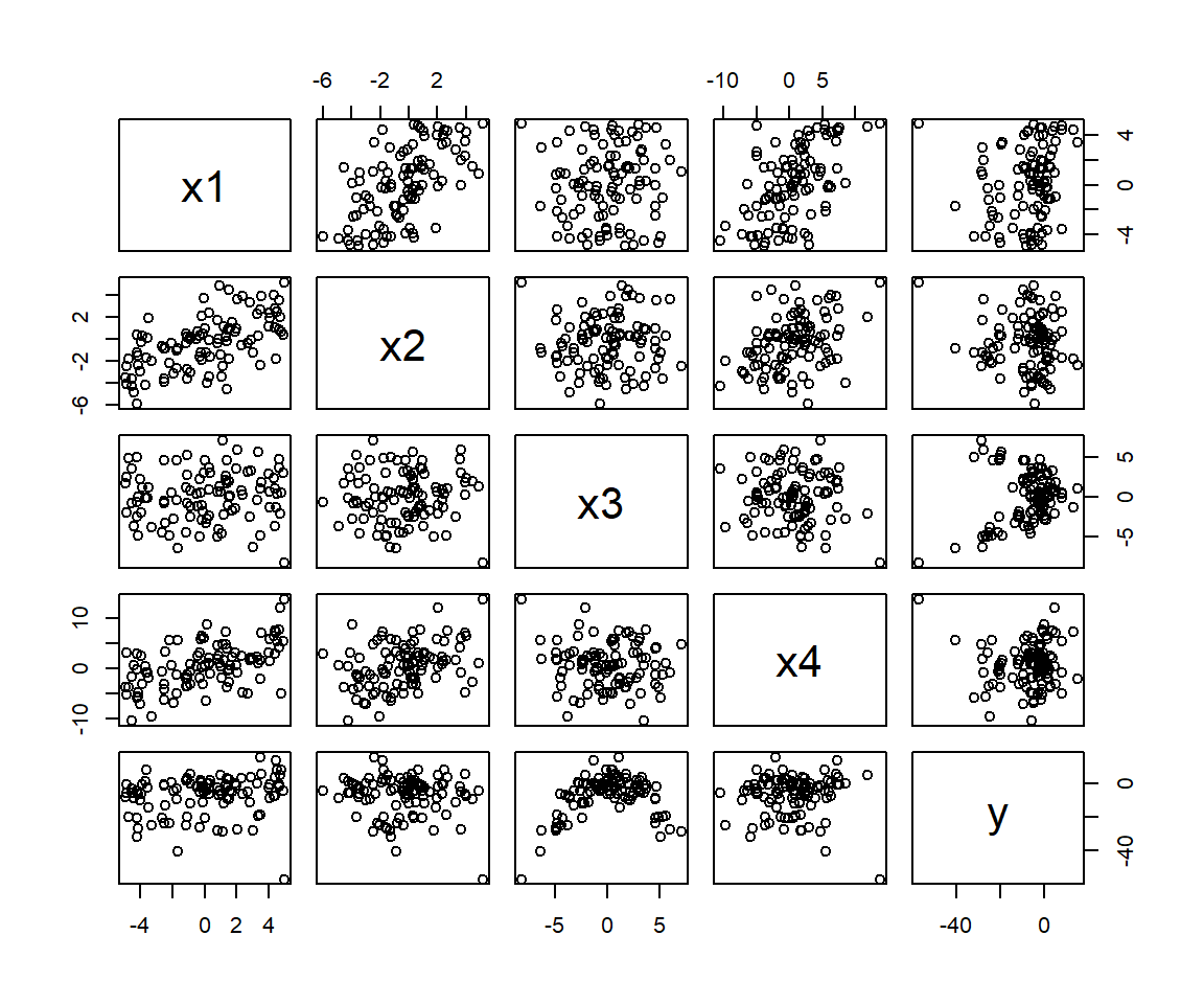
FIGURE 3.10: Pairwise scatterplot of the predictors in the partialr data set in the Data4ecologists package (J. Fieberg, 2021). These data were simulated so that y has a positive association with x1, a negative association with x2 (which is also negatively correlated with x1), a quadratic relationship with x3, and a spurious relationship with x4 (due to its correlation with x1).
First, note that whenever predictor variables are correlated, as they will be in any observational data set, regression coefficients will change when we add or drop predictors from a model model as these correlated variables “compete” to predict variance in the response variables (see e.g., Table 3.2). The magnitude and direction of these changes will depend on the sign and strength of the correlations among the different predictor variables (see Sections 6 and 7; Fieberg & Johnson, 2015) [add link to mulicollinearity chapter and simulation]. Thus, choosing an appropriate model can be challenging and should ideally be informed by one’s research question and an assumed Directed Acyclical Graph (DAG) capturing assumptions about how the world works (i.e., causal relationships between the predictor variables and the response variable; see Section 7).
lmx1.y <- lm(y ~ x1, data=partialr)
lmx2.y <- lm(y ~ x2, data=partialr)
lmx3.y <- lm(y ~ x3, data=partialr)
lmx4.y <- lm(y ~ x4, data=partialr)
lmxall.y <- lm(y ~ x1 + x2 + x3 + x4, data=partialr)| Model 1 | Model 2 | Model 3 | Model 4 | Model 5 | |
|---|---|---|---|---|---|
| (Intercept) | -7.359 | -7.479 | -7.384 | -7.300 | -7.865 |
| x1 | 0.692 | 1.562 | |||
| x2 | -0.495 | -1.505 | |||
| x3 | 0.925 | 0.842 | |||
| x4 | -0.025 | -0.210 |
For now, let’s assume we have chosen to focus on the model containing all four predictor variables and we want to display the effect of x1 after accounting for the other predictors in the model using an added-variable plot. Let’s walk through the steps of this process:
- Regress \(Y\) against \(X_{-k}\) (i.e., all predictors except
x1).
- Regress \(X_k\) against all other predictors (\(X_{-k}\)).
- Plot the residuals from [1] against the residuals from [2] along with a regression line relating these two sets of residuals. We also add a regression line through the origin with the slope coefficient for
x1from the original regression.
plot(resid(lm.x1.allotherx), resid(lm.nox1.y),
     xlab="E(X1 | X2, X3, X4)", ylab= "E(Y | X2, X3, X4)")
abline(c(0,coef(lmxall.y)[2]), col="red", lty=2, lwd=3)
(lmpartial<-lm(resid(lm.nox1.y)~resid(lm.x1.allotherx)-1))
##
## Call:
## lm(formula = resid(lm.nox1.y) ~ resid(lm.x1.allotherx) - 1)
##
## Coefficients:
## resid(lm.x1.allotherx)
## 1.562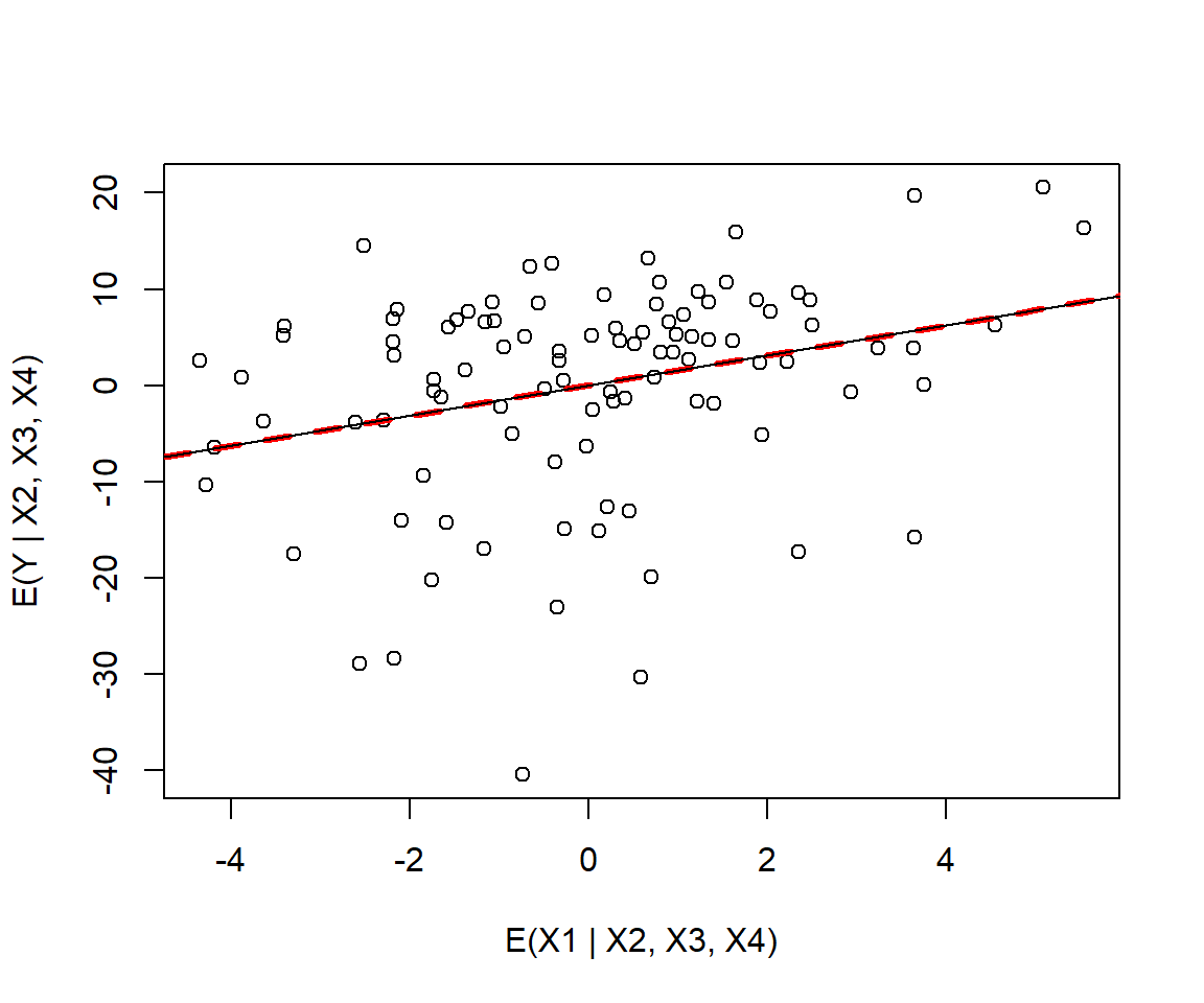
FIGURE 3.11: Added variable plot for variable x1 in the partialr data set.
We see that the slope from the original regression is equivalent to the slope of the regression line relating the residuals from [1] to the residuals from [2].
Rather than construct similar plots for the other variables, we will use the avPlots function in the car package to produce the full suite of added variable plots:
partialr data set in the Data4Ecologists package (J. Fieberg, 2021) calculated using the avplots function in the car package (Fox & Weisberg, 2019a).
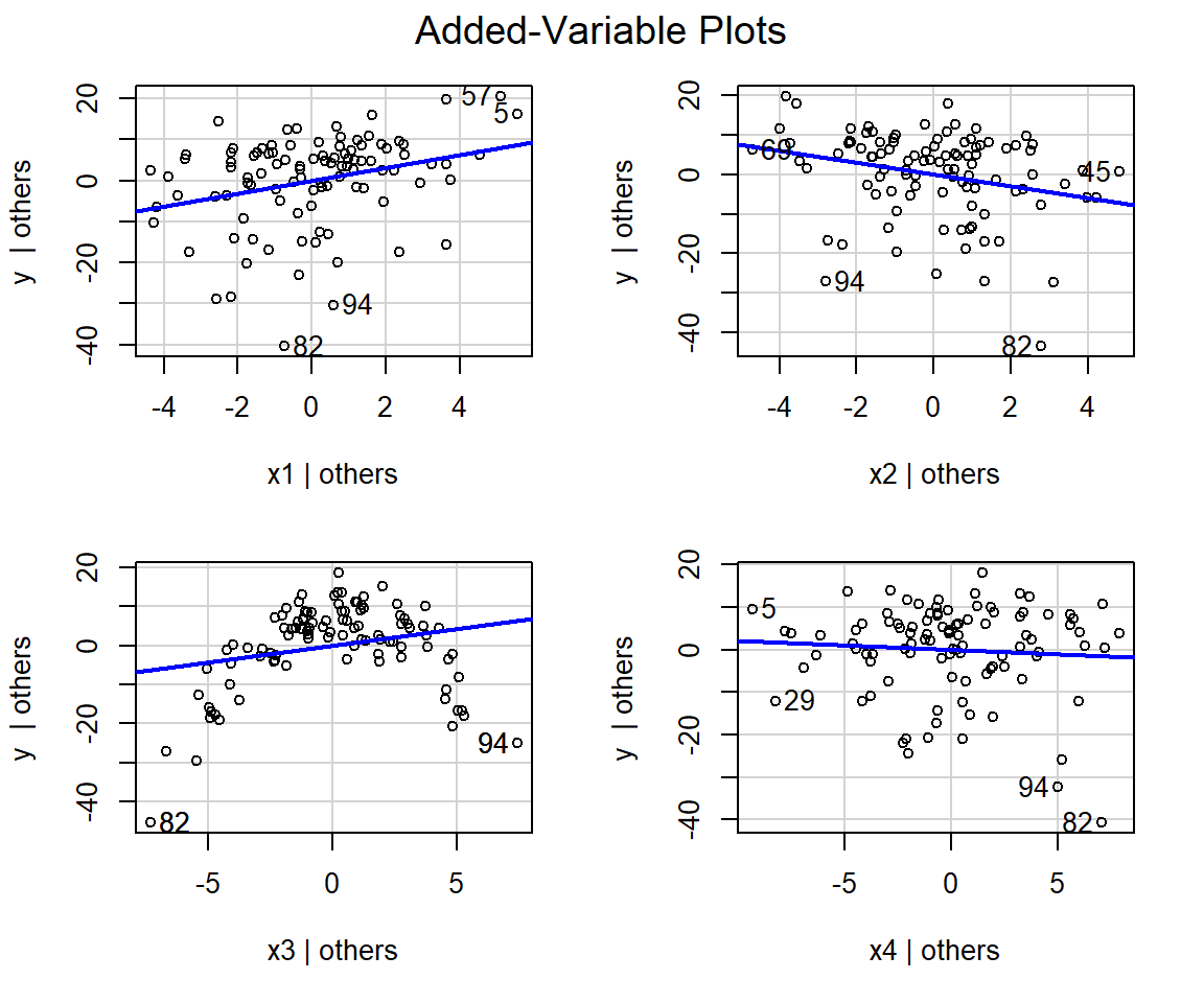
FIGURE 3.12: (ref:parresidplotcar)
We see that the slope of the line is near 0 in the plot for x4 (lower right panel of Figure 3.12), suggesting that x4 provides little to no additional information useful for predicting y that is not already contained in the other predictor variables. Further, in the plot for x3 (lower-left panel of Figure 3.12), we see that it has a clear non-linear relationship with y even after accounting for the effects of x1, x2, and x4. Thus, we may want to add a quadratic term or use splines to relax the linearity assumption for this variable (see Section 4).
In summary, added-variable plots depict the slope and the scatter of points around the partial regression line in an analogous way to bi-variate plots in simple linear regression. These plots can be helpful for:
- visualizing the effect of predictor variables (given everything else already in the model)
- diagnosing whether some variables have a non-linear relationship with the response variable
- identifying potential influential points and outliers (
avPlotshighlights these with the row number in the data set)
One downside to added-variable plots is that the scales on the x- and y-axis do not match the scales of the original variables in the regression model.
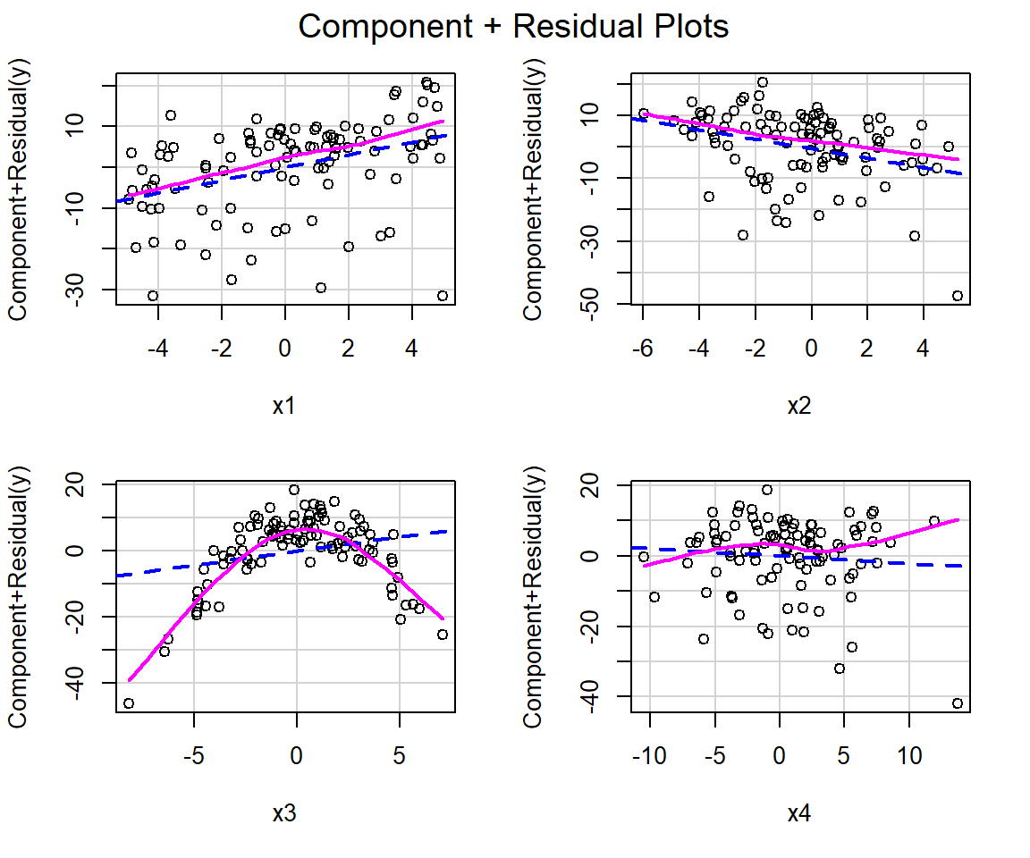
3.13.2 Component + residual plots or partial residual plots
Component + residual plots, which are sometimes referred to as partial residual plots, offer a slightly different visualization by plotting:
\[X_i\hat{\beta}_i + \hat{\epsilon}_i \mbox{ versus } X_i, \text{where}\].
\(X_i\) is the \(i^{th}\) predictor variable and is the variable of interest. As shown, below, \(X_i\hat{\beta}_i + \hat{\epsilon}\) represents the part of \(Y\) explained by \(X_i\) that is not already explained by all the other predictors:
\[Y-\sum_{j \ne i}X_j\hat{\beta}_j = \hat{Y} + \hat{\epsilon} - \sum_{j \ne i}X_j\hat{\beta}_j = X_i\hat{\beta}_i + \hat{\epsilon}\]
There are a number of options in R for creating component + residual plots (see Section 3.13). This approach can be easily generalized to more complicated models that allow for non-linear relationships (e.g., quadratic terms), by replacing \(X_i\hat{\beta}_i\) with multiple terms corresponding to the columns in the design matrix associated with the \(i^{th}\) explanatory variables; however, component + residual plots are not appropriate if you include interactions in the model. Moya-Laraño & Corcobado (2008) suggest that component + residual plots are sometimes better than added variable plots at diagnosing non-linearities, but they are not as good as added-variable plots at depicting the amount of variability explained by each predictor (given everything else in the model).
Below, we demonstrate how to construct component + residual plots using the crPlots function in the car package.
3.13.3 Effect plots
Another way to visualize fitted regression models is to form effect plots using what Lüdecke (2018) refers to as either adjusted or marginal means. Plots of adjusted means are formed using predictions where a focal variable is varied over its range of observed values, while all non-focal variables are set to constant values (e.g., at their means or modal values). Marginal means are formed in much the same way, except that predictions are averaged across different levels of each categorical variable. These two types of means are equivalent if there are no categorical predictors in the model.
Marginal means can be calculated using the effects function in the effects package and then plotted. Alternatively, we can use the ggeffect function in the ggeffects package (Lüdecke, 2018) to format the output and create plots using ggplot2 (Wickham, 2016). Adjusted means can be created using the ggpredict function in the ggeffects package or the visreg function in the visreg package (Breheny & Burchett, 2013). The visreg package also provides an option for producing contrast plots, which compare adjusted means to predictions obtained by setting all predictors (including the focal predictor) to specific reference values.
Below, we briefly illustrate the ggeffect and ggpredict functions using the RIKZdat data set and our linear model containing week and NAP (but not their interaction). If we use ggpredict or ggeffect with the argument terms = c("NAP", "week.cat"), we get predictions for a range of NAP values associated with each week. The output of these functions is a list with an associated print function that provides nicely formatted output.
## # Predicted values of Richness
##
## # week.cat = 1
##
##   NAP | Predicted |         95% CI
## ----------------------------------
## -1.40 |     14.55 | [12.28, 16.82]
## -0.60 |     12.73 | [10.76, 14.70]
##  0.00 |     11.37 | [ 9.46, 13.28]
##  0.80 |      9.55 | [ 7.46, 11.64]
##  2.20 |      6.37 | [ 3.48,  9.27]
##
## # week.cat = 2
##
##   NAP | Predicted |        95% CI
## ---------------------------------
## -1.40 |      6.92 | [ 4.56, 9.28]
## -0.60 |      5.11 | [ 3.24, 6.97]
##  0.00 |      3.74 | [ 2.12, 5.36]
##  0.80 |      1.93 | [ 0.34, 3.52]
##  2.20 |     -1.25 | [-3.51, 1.00]
##
## # week.cat = 3
##
##   NAP | Predicted |         95% CI
## ----------------------------------
## -1.40 |      8.37 | [ 6.04, 10.70]
## -0.60 |      6.55 | [ 4.71,  8.39]
##  0.00 |      5.19 | [ 3.58,  6.80]
##  0.80 |      3.37 | [ 1.78,  4.97]
##  2.20 |      0.19 | [-2.09,  2.48]
##
## # week.cat = 4
##
##   NAP | Predicted |        95% CI
## ---------------------------------
## -1.40 |     11.95 | [8.65, 15.25]
## -0.60 |     10.14 | [7.21, 13.07]
##  0.00 |      8.77 | [6.01, 11.53]
##  0.80 |      6.96 | [4.25,  9.66]
##  2.20 |      3.78 | [0.68,  6.87]
We can then use a built in plot function to visualize these predictions with partial residuals overlaid by adding residuals = TRUE (Figure 3.14).
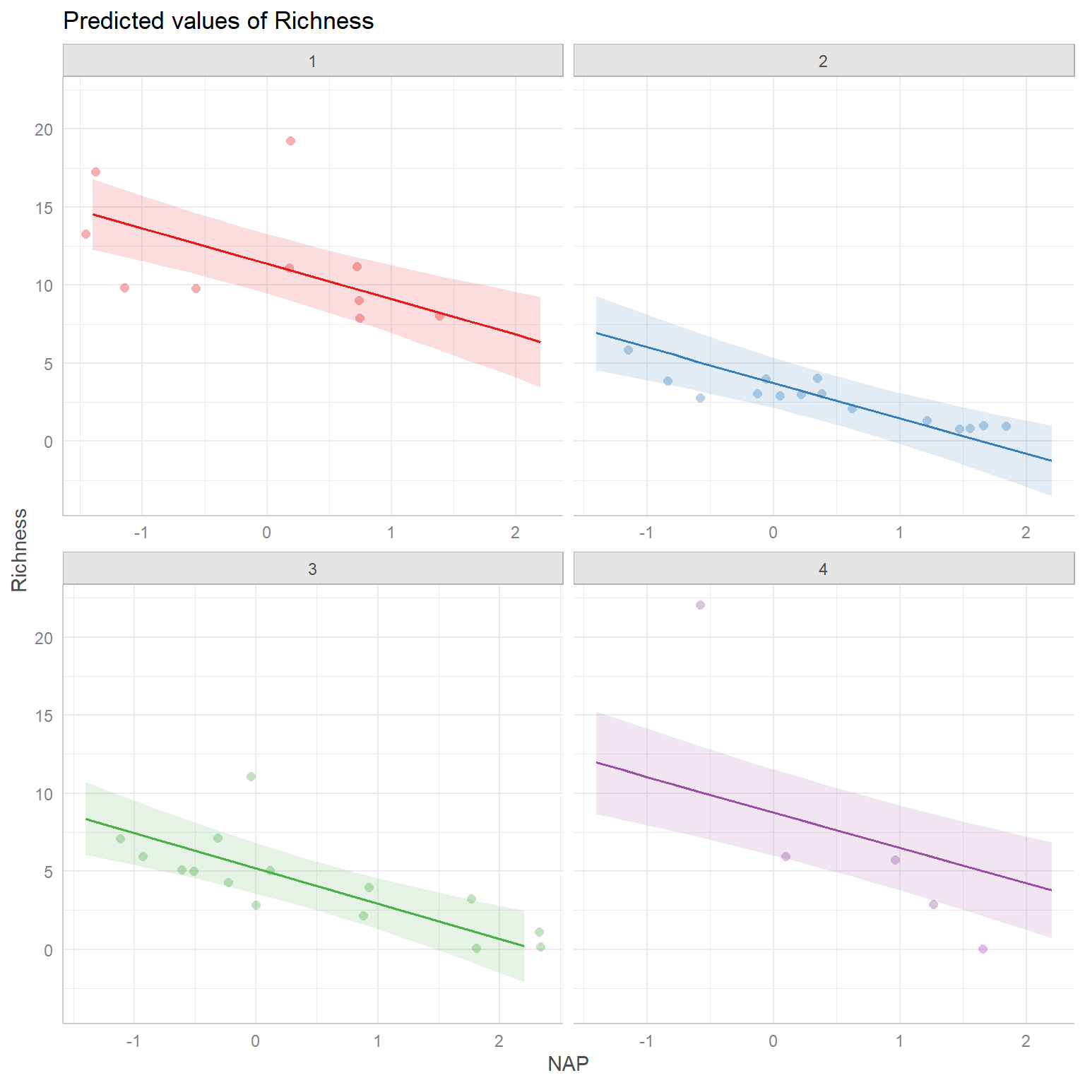
FIGURE 3.14: Effect plot created using ggpredict showing adjusted means for different combinations of week.cat and NAP along with partial residuals.
Alternatively, if we want to create a plot just for NAP, we can use either ggpredict (for adjusted means) or ggeffect (for marginal means).
## # Predicted values of Richness
##
##   NAP | Predicted |         95% CI
## ----------------------------------
## -1.40 |     14.55 | [12.35, 16.75]
## -1.00 |     13.64 | [11.61, 15.66]
## -0.40 |     12.28 | [10.40, 14.15]
##  0.00 |     11.37 | [ 9.51, 13.22]
##  0.40 |     10.46 | [ 8.55, 12.37]
##  0.80 |      9.55 | [ 7.52, 11.58]
##  1.20 |      8.64 | [ 6.44, 10.85]
##  2.20 |      6.37 | [ 3.56,  9.18]
##
## Adjusted for:
## * week.cat = 1## # Predicted values of Richness
##
## NAP | Predicted | 95% CI
## ----------------------------------
## -1.40 | 9.66 | [ 7.78, 11.54]
## -1.00 | 8.75 | [ 7.19, 10.31]
## -0.40 | 7.39 | [ 6.24, 8.53]
## 0.00 | 6.48 | [ 5.52, 7.44]
## 0.40 | 5.57 | [ 4.67, 6.47]
## 0.80 | 4.66 | [ 3.67, 5.66]
## 1.20 | 3.75 | [ 2.55, 4.96]
## 2.20 | 1.48 | [-0.49, 3.45]ggpredict forms predictions where week.cat is set to 1 (its reference value), whereas ggeffect generates predictions for each week, then averages these predictions, weighted by the proportion of observations in each week (for more on these calculations, see Section 16.5.4). As a result, the absolute values of the predictions will differ even though the effect of NAP will look similar when we visualize the output (i.e., the slope of the depicted line is the same in both panels of Figure 3.15)
library(patchwork)
p1 <- plot(padj, residuals = TRUE, facet = TRUE)
p2 <- plot(pm, residuals = TRUE, facet = TRUE)
p1 + p2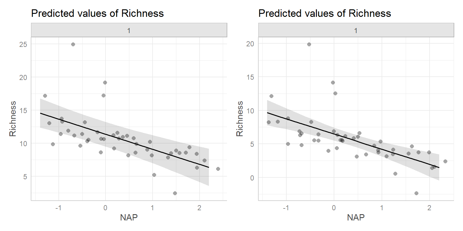
FIGURE 3.15: Effect plots created using ggpredict (left) and ggeffect (right) showing adjusted and marginal means, with partial residuals.
Note: the normality assumption is required for small data sets, but the Central Limit Theorem (CLT) guarantees that sampling distribution for a difference in sample means will be approximately Normally distributed for large samples; a common rule is that we need roughly 30 observations in both groups for the CLT to apply↩
Note: there are other variations on the t-test that could be applied if the variances of the two groups are not assumed to be equal↩
Importantly, I want to formally recognize that a binary framework for sexual identification does not encompass everyone’s experience or identity and that more inclusive categories should be considered in human-subject research.↩
In fact, many more connections can be made between linear regression models and common statistical methods; see e.g., https://lindeloev.github.io/tests-as-linear/.↩
We refer to expected
Richnesshere to signify that we need to average over \(\epsilon_i\)↩Note that our species richness measure is just the count of species on the sampled beach↩
It is common with experimental data to test for significant interactions prior to testing main effects of individual predictors. For observational data, however, it is prudent to be more cautious. A sensible approach is often to include interactions only when they can be justified a priori based on biological grounds. Here, for illustrative purposes only, we will explore a model that includes an interaction between
NAPandweek.cat, but we suspect it would be difficult to motivate the need for this interaction, and the researchers did not design their study to test for it↩There is also a type II sums of squares that is most relevant to models that also include one or more interaction terms. We will not consider them here↩