Chapter 16 Logistic regression
Learning objectives
- Be able to formulate, fit, and interpret logistic regression models appropriate for binary data using R and JAGS
- Be able to compare models and evaluate model fit
- Be able to visualize models using effect plots
- Be able to describe statistical models and their assumptions using equations and text and match parameters in these equations to estimates in computer output
16.1 Introduction to logistic regression
Logistic regression is used to relate a binary response variable, \(Y_i\) (i.e., a variable that can take on only 1 of two values, e.g., Yes/No, Alive/Dead, Infected/Not-infected), to a set of explanatory variables, \(X_i = (X_{i,1}, X_{i,2}, \ldots, X_{i,p})\). The model assumes \(Y_i\) follows a Bernoulli distribution with probability of “success” (i.e.,, \(P(Y_i = 1)\) that depends on predictors, \(X_i\), via the following set of equations:
\[Y_i | X_i \sim \text{Bernoulli}(p_i)\]
\[\log\left(\frac{p_i}{1-p_i}\right) = \text{logit}(p_i) = \beta_0 + \beta_1 X_{1,i}+ \ldots \beta_p X_{p,i}\]
The quantity \(\Large\frac{p}{1-p}\) is referred to as the odds of success, and the link function, \(\log \Big(\frac{p}{1-p}\Big)\), is referred to as logit. Thus, we can describe our model in the following ways:
- We are modeling \(\log \Big(\frac{p}{1-p}\Big)\) as a linear function of \(X_1, \dots, X_p\).
- We are modeling the logit of \(p\) as a linear function of \(X_1, \dots, X_p\).
- We are modeling the log odds of “success” (defined as \(Y_i = 1\)) as a linear function of \(X_1, \dots, X_p\).
To determine \(E[Y_i|X_i] = p_i\), we need to apply the inverse-logit transformation:
\[p_i = g^{-1}(\beta_0 + \beta_1X_{1,i}+\ldots \beta_pX_{p,i}) = \frac{\exp(\beta_0 + \beta_1X_{1,i}+\ldots \beta_pX_{p,i})}{1+\exp(\beta_0 + \beta_1X_{1,i}+\ldots \beta_pX_{p,i})}.\]
As the linear predictor, \(\log \Big(\frac{p}{1-p}\Big) = \normalsize \beta_0 + \beta_1X_{1,i}+\ldots \beta_pX_{p,i}\), ranges between \(-\infty\) and \(\infty\), the odds = \(\exp\Big(\frac{p}{1-p}\Big)\) ranges between 0 and \(\infty\), and \(p\) is constrained to be between 0 and 1 (Table 16.1).
| log odds \(= \log\Big(\frac{p}{1-p}\Big)\) | -6.907 | -1.386 | 0.0 | 1.386 | 6.907 |
| odds \(= \frac{p}{1-p}\) | 0.001 | 0.250 | 1.0 | 4.000 | 999.000 |
| p | 0.001 | 0.200 | 0.5 | 0.800 | 0.999 |
We can gain further insights into the model by plotting \(p_i\) as a function of \(X_i\) for a logistic regression model with a single continuous predictor and associated intercept and slope parameters, \(\beta_0\) and \(\beta_1\), respectively (Figure 16.1). The sign of \(\beta_1\) determines whether \(p\) increases or decreases as \(X_i\) increases, and its magnitude controls how quickly \(p_i\) transitions from 0 to 1
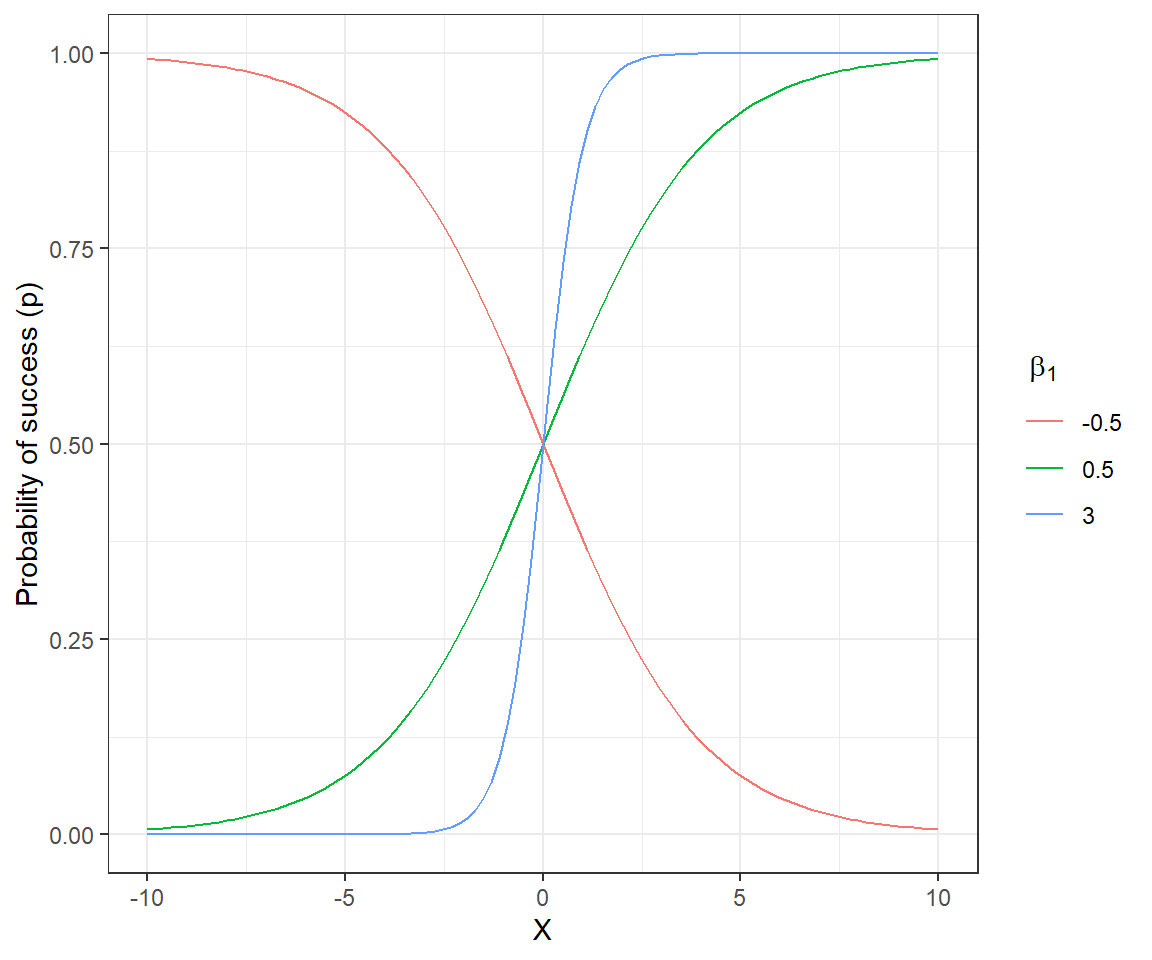
FIGURE 16.1: Probability of success for different slope coefficients in a logistic regression model with a single continuous predictor and \(\beta_0 = 0\).
The intercept \(\beta_0\) controls the height of the curve when \(X_i=0\). For the curves depicted in Figure 16.1, \(\beta_0 = 0\). Thus, \(E[Y_i |X_i=0] = \frac{exp(\beta_0)}{1+exp(\beta_0)} = 1/2\).
16.2 Parameter Interpretation: Application to moose detection data
In Section 11, we considered data collected by the MN DNR to estimate the probability of detecting a moose when flying a helicopter survey (Giudice et al., 2012). The probability of detecting a moose will depend on where the moose is located (e.g., the amount of cover that shields the moose from view, termed visual obstruction (or VOC); Fig. 16.2). If we model the probability of detection as a function of VOC, we can then adjust counts of observed animals in future surveys that also record this information, providing a formal method for estimating moose abundance that accounts for imperfect detection (Fieberg, 2012; Fieberg, Alexander, Tse, & St. Clair, 2013; ArchMiller, Dorazio, Clair, & Fieberg, 2018). We might also want to consider whether detection probabilities vary by observer (a categorical variable) or whether detection probabilities varied among the four years of data collection.
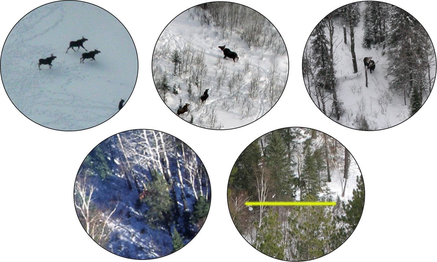
FIGURE 16.2: Observations of moose in Minnesota with a circular field of view used to measure the degree of visual obstruction. Photos by Mike Schrage, Fond du Lac Resource Management Division.
Let’s read in a data set with the observations recording whether each moose was observed or not along with potential covariates for modeling the probability of detection. The data are contained in the SightabilityModel package (Fieberg, 2012) and can be accessed using:
## Warning: package 'SightabilityModel' was built under R version 4.1.1## 'data.frame': 124 obs. of 4 variables:
## $ year : int 2005 2005 2005 2005 2005 2005 2005 2005 2005 2005 ...
## $ observed: int 1 1 0 0 0 0 1 1 1 1 ...
## $ voc : int 20 85 80 75 70 85 20 10 10 70 ...
## $ grpsize : int 4 2 1 1 1 1 1 2 2 2 ...The data set in this package contains a small subset of the variables that could be used to model detection probabilities (see Giudice et al., 2012 for a discussion relative to selecting an appropriate model). We will focus on the relationship between detection and visual obstruction measurements using the variables observed and voc, respectively. Note that the variable observed is binary:
\[observed_{i} = \left\{ \begin{array}{ll} 1 & \mbox{if the radiocollared moose was detected}\\ 0 & \mbox{if the radiocollared moose was not detected} \end{array} \right.\]
In Figure 16.3, we use a smoother to visualize overall trends in detection probabilities relative to voc. As expected, we see that detection probabilities decrease as the amount of screening cover increases. We could fit a linear regression model to the data. However, this approach would fail to capture several characteristics of the data:
- Detection probabilities must necessarily fall between 0 and 1.
- The observations do not have have constant variance (recall the variance of a Bernoulli random variable = \(p(1-p)\), which will be at its highest value when \(p=0.5\)).
ggplot(exp.m, aes(voc,observed))+theme_bw()+
    geom_point(position = position_jitter(w = 2, h = 0.05), size=3) +
    geom_smooth(colour="red") + xlab("Visual Obstruction") +
    ylab("Detection = 1")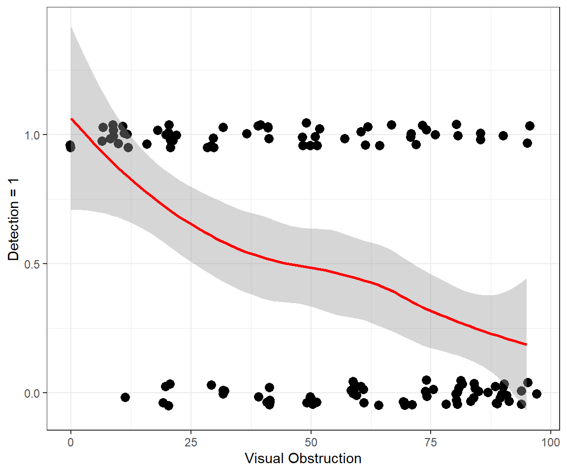
FIGURE 16.3: Detection of moose as a function of the amount of visual obstruction within an approximate 10m radius of the moose.
Letting \(Y_i = observed_i\), and \(X_i = voc_i\), we can specify a logistic regression model for the moose data using the following set of equations:
\[Y_i | X_i \sim Bernouli(p_i)\]
\[logit(p_i) = \log\left(\frac{p_i}{1-p_i}\right) = \beta_0 + \beta_1 voc_i\]
By default, glm will use a logit link when specifying family=binomial(), but other links are possible. Like other regression models we’ve seen, we can use the summary function to view the estimated coefficients, their standard errors, and hypothesis tests for whether the coefficients are 0 (versus an alternative that they are not 0):
##
## Call:
## glm(formula = observed ~ voc, family = binomial(), data = exp.m)
##
## Deviance Residuals:
##     Min       1Q   Median       3Q      Max
## -1.8056  -0.9071  -0.6218   0.9745   1.8647
##
## Coefficients:
##              Estimate Std. Error z value Pr(>|z|)
## (Intercept)  1.759933   0.460137   3.825 0.000131 ***
## voc         -0.034792   0.007753  -4.487 7.21e-06 ***
## ---
## Signif. codes:  0 '***' 0.001 '**' 0.01 '*' 0.05 '.' 0.1 ' ' 1
##
## (Dispersion parameter for binomial family taken to be 1)
##
##     Null deviance: 171.61  on 123  degrees of freedom
## Residual deviance: 147.38  on 122  degrees of freedom
## AIC: 151.38
##
## Number of Fisher Scoring iterations: 4
We see that the log-odds of detection decreases by -0.035 as we increase voc by 1 unit (i.e., for every increase of 1% visual obstruction). Alternatively, it is common to report effect sizes in terms of a change in odds. The odds of detection is given by:
\[\frac{p_i}{1-p_i}= \exp(\beta_0+\beta_1voc_i) = e^{\beta_0}e^{\beta_1voc_i}\]
Thus, if we increase voc by 1 unit, we increase the odds by \(e^{\beta_1}\). To calculate a confidence interval for the change in odds associated with a 1 unit increase in a predictor variable, it is common to calculate a confidence interval for \(\beta_1\) and then exponentiate the limits (similar to what we saw for Poisson regression). Again, we can rely on large sample theory for Maximum Likelihood estimators, \(\hat{\beta}\sim N(\beta, I^{-1}(\beta))\), and the output from the summary of the glm model to calculate a 95% confidence interval for \(\beta_1\) and also for the change in odds:
beta1 <- coef(mod1)[2]
SEbeta1 <- sqrt(diag(vcov(mod1)))[2]
oddsr <- exp(beta1)
CI_beta <- beta1 + c(-1.96, 1.96)*SEbeta1
CI_odds <- exp(CI_beta)
estdata <- data.frame(beta1 = beta1, SEbeta1 = SEbeta1,
           LCL_beta = CI_beta[1], UCL_beta = CI_beta[2], oddsratio  = oddsr,
           LCL_odds = CI_odds[1], UCL_odds = CI_odds[2])
colnames(estdata) <- c("$\\widehat{\\beta}_1$", "$SE(\\widehat{\\beta}_1)$",
                             "Lower 95\\% CL", "Upper 95\\% CL", "$\\exp(\\beta_1)$",
                             "Lower 95\\% C", "Upper 95\\% CL")
kable(round(estdata,3), booktabs = TRUE, escape = FALSE)| \(\widehat{\beta}_1\) | \(SE(\widehat{\beta}_1)\) | Lower 95% CL | Upper 95% CL | \(\exp(\beta_1)\) | Lower 95% C | Upper 95% CL | |
|---|---|---|---|---|---|---|---|
| voc | -0.035 | 0.008 | -0.05 | -0.02 | 0.966 | 0.951 | 0.981 |
Alternatively, we could calculate profile-likelihood based confidence intervals by inverting the likelihood ratio test (Section 10.9). Recall, profile-likelihood intervals include all values, \(\widetilde{\beta}\) for which we would not reject the null hypothesis \(H_0: \beta=\widetilde{\beta}\). In small samples, profile likelihood intervals should perform better than the Normal-based intervals, and thus, this is the default approach used by the function confint:
## Waiting for profiling to be done...## 2.5 % 97.5 %
## (Intercept) 0.89794673 2.71375978
## voc -0.05082098 -0.02025314## 2.5 % 97.5 %
## (Intercept) 2.4545581 15.0858887
## voc 0.9504488 0.9799506Both confidence intervals are similar in this case. If confidence limits for \(\beta\) do not include 0 or confidence limits for \(\exp(\beta)\) do not include 1, then the results are statistically significant at the \(\alpha = 0.05\) level.
We can also use tab_model in the sjPlot library or the modelsummary function in the modelsummary package to calculate a table of effect sizes for our model (Table 16.2). By default, tab_model reports effect sizes in terms of odds, labeled Odds Ratios. We can can also calculate odds ratios by adding the argument exponentiate = TRUE when calling the modelsummary function (Table 16.2).
modelsummary(list("Logistic regression" = mod1),
             exponentiate = TRUE, gof_omit = ".*", estimate  = "{estimate} ({std.error})",
             statistic=NULL,
             coef_omit = "SD",
             title = "Odds ratios (SE) from the logistic regression model fit
to the moose detection data.") | Logistic regression | |
|---|---|
| (Intercept) | 5.812 (0.460) |
| voc | 0.966 (0.008) |
To understand why \(\exp(\hat{\beta})\) is referred to as an odds ratio, consider the ratio of odds for two observations that differ only in voc with \(voc_2 = voc_1+1\). The ratio of odds for observation 2 relative to observation 1 is given by:
\[\frac{\frac{p_2}{1-p_2}}{\frac{p_1}{1-p_1}} = \frac{e^{\beta_0}e^{\beta_1voc_2}}{e^{\beta_0}e^{\beta_1voc_1}} = \frac{e^{\beta_1(voc_1+1)}}{e^{\beta_1voc_1}}= e^{\beta_1}\]
What about the intercept? The intercept gives the log-odds of detection when voc = 0 (i.e., when moose are completely in the open). We can also use the plogis function in R to calculate the inverse-logit transform, \(g^{-1}(\beta_0) = \frac{exp(\beta_0)}{1+exp(\beta_0)}\), which provides an estimate of the probability of success when all covariates are equal to 0 (or when all covariates are set to their means if we use centered and scaled predictors):
## (Intercept)
##   0.8532013
Thus, the model predicts there is an 85% chance of detecting a moose when it is completely in the open (i.e., when voc = 0).
Lastly, we can visualize the model using `ggplot using stat_smooth (Figure 16.4).
ggplot(exp.m, aes(voc,observed)) + theme_bw() +
    geom_point(position = position_jitter(w = 2, h = 0.05), size=3) +
    xlab("Visual Obstruction") +
    stat_smooth(method="glm", method.args = list(family = "binomial") )+
ylab("Detection = 1") 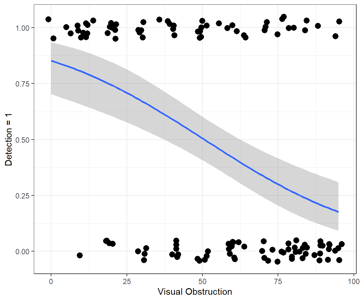
FIGURE 16.4: Fitted logistic regression model relating detection probabilities to the amount of visual obstruction.
16.2.1 Model with continuous and categorical variables
Lets now consider a second model, where we also include year of the observation as a predictor.
exp.m$year <- as.factor(exp.m$year)
mod2 <- glm(observed ~ voc + year, data = exp.m, family = binomial())
summary(mod2)
Call:
glm(formula = observed ~ voc + year, family = binomial(), data = exp.m)

Deviance Residuals:
    Min       1Q   Median       3Q      Max
-1.9351  -0.8411  -0.4561   0.9493   1.8680

Coefficients:
             Estimate Std. Error z value Pr(>|z|)
(Intercept)  2.453203   0.622248   3.942 8.06e-05 ***
voc         -0.037391   0.008199  -4.560 5.11e-06 ***
year2006    -0.453862   0.516567  -0.879   0.3796
year2007    -1.111884   0.508269  -2.188   0.0287 *
---
Signif. codes:  0 '***' 0.001 '**' 0.01 '*' 0.05 '.' 0.1 ' ' 1

(Dispersion parameter for binomial family taken to be 1)

    Null deviance: 171.61  on 123  degrees of freedom
Residual deviance: 142.23  on 120  degrees of freedom
AIC: 150.23

Number of Fisher Scoring iterations: 4
Again, R uses effects coding by default. This provides another opportunity to revisit design matrices from Section 3 as well as further test our ability to interpret the regression coefficients when we include multiple predictor variables.
Think-Pair-Share: How can we interpret the coefficients in our model with year and voc?
Since we did not included an interaction between voc and year, we have assumed the effect of voc is the same in all years. We can interpret the effect of voc in the same way as in Section 16.2, except we must now tack on the phrase while holding year constant. I.e., the log odds of detection changes by 0.037 and the odds of detection by 0.96 for every 1 unit increase in voc while holding year constant.
What about the three coefficients associated with the year variables that R created? These coefficients provide estimates of differences in the log odds of detection between each listed year and 2005 (the reference level), while holding voc constant. And, if we exponentiate these coefficients, we get ratios of odds (i.e., odds ratios) between each year and 2005 (Table 16.3), while holding voc constant.
| Logistic regression | |
|---|---|
| (Intercept) | 11.626 (0.622) |
| voc | 0.963 (0.008) |
| year2006 | 0.635 (0.517) |
| year2007 | 0.329 (0.508) |
Thus, for example, we can conclude that the odds of detection were 1/0.635 = 1.57 times higher in 2005 than 2006 if we hold voc constant.
16.2.2 Interaction model
What if we were to include an interaction between voc and year?
##
## Call:
## glm(formula = observed ~ voc * year, family = binomial(), data = exp.m)
##
## Deviance Residuals:
##     Min       1Q   Median       3Q      Max
## -1.8622  -0.9865  -0.3089   0.9818   2.0384
##
## Coefficients:
##              Estimate Std. Error z value Pr(>|z|)
## (Intercept)   1.53466    0.83338   1.841   0.0656 .
## voc          -0.02224    0.01287  -1.728   0.0839 .
## year2006      0.35841    1.20786   0.297   0.7667
## year2007      0.55335    1.13559   0.487   0.6261
## voc:year2006 -0.01310    0.02002  -0.655   0.5127
## voc:year2007 -0.03151    0.01983  -1.589   0.1121
## ---
## Signif. codes:  0 '***' 0.001 '**' 0.01 '*' 0.05 '.' 0.1 ' ' 1
##
## (Dispersion parameter for binomial family taken to be 1)
##
##     Null deviance: 171.61  on 123  degrees of freedom
## Residual deviance: 139.60  on 118  degrees of freedom
## AIC: 151.6
##
## Number of Fisher Scoring iterations: 4Think-Pair-Share: How can we interpret the coefficients in the above model?
The year2006 and year2007 terms provide estimates of differences in intercepts between each listed year and the reference level (2005 in this case) and the voc:year2006 and voc:year2007 terms provide estimates of differences in slopes between each listed year and the reference level year. If this is not clear, it would help to review Section 3. You might also consider trying to write out the design matrix for a few observations in the data set that come from different years. You could then check your understanding using the model.matrix function. Try writing out the design matrix for the following observations:
##     voc year
## 37   20 2005
## 73   10 2007
## 89   60 2006
## 110  85 2007
Check your answer by typing:
16.3 Evaluating assumptions and fit
We can use similar methods as seen in Section 15.3 to evaluate model fit.
16.3.1 Residual plots
As discussed in Section 15.3.1, there are multiple types of residuals (standard, Pearson, deviance) that we might consider using to evaluate model fit. Below, we use the residualPlots function in the car library to create plots of Pearson residuals versus model predictors and versus fitted values (Figure 16.5).
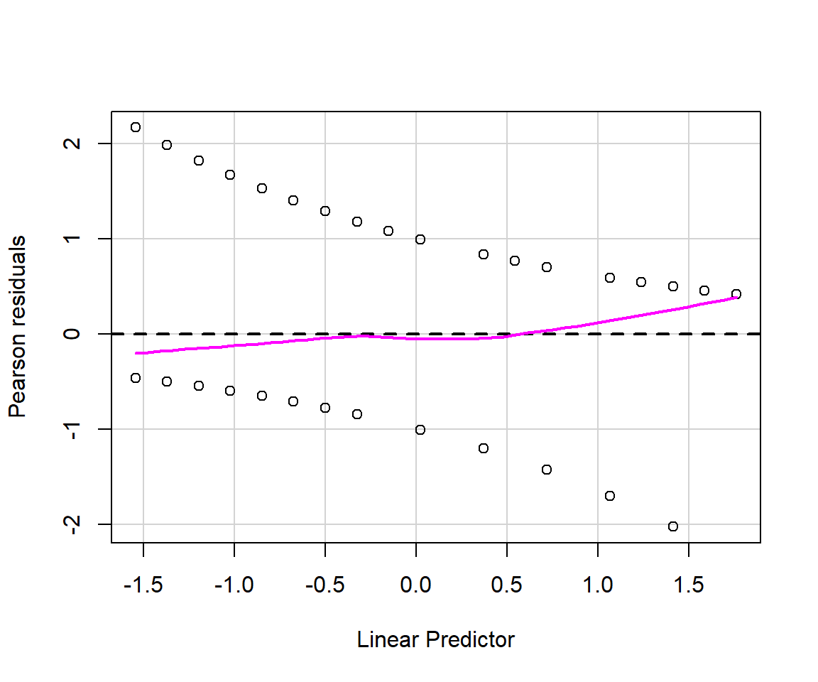
FIGURE 16.5: Residual plots for the logistic regression model fit to data from Moose in Minnesota.
The residuals for binary data always look weird since \(Y_i\) can only take on the values of 0 and 1. Thus, it is important to focus on the smooth line to see if there is any patterning. Alternatively, it can be beneficial to create binned residual plots by “dividing the data into categories (bins) based on their fitted values, and then plotting the average residual versus the average fitted value for each bin.” (Gelman & Hill, 2006). The binned_residual function in the performance package will do this for us (Figure 16.6). It also provides error bounds and colors binned residuals that fall outside these bounds to help easily visualize whether the model provides a poor fit to the data.
Warning: About 91% of the residuals are inside the error bounds (~95% or higher would be good).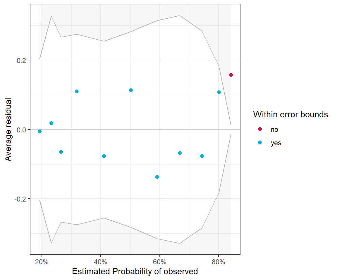
FIGURE 16.6: Binned residual plot for the logistic regression model containing only voc.
16.3.2 Goodness-of-fit test
We can easily adapt the general approach for testing goodness-of-fit from Sections 13.3 and 15.3.5 to logistic regression models. Again, we will consider the sum of Pearson residuals as our goodness-of-fit statistic:
\[\chi^2_{n-p} = \sum_{i=1}^n\frac{(Y_i-E[Y_i|X_i])^2}{Var[Y_i|X_i]}\]
For binary data analyzed using logistic regression, we have:
- \(E[Y_i|X_i] = p_i\) = \(\Large \frac{exp(\beta_0 + \beta_1x_1+\ldots \beta_kx_k)}{1+exp(\beta_0 + \beta_1x_1+\ldots \beta_kx_k)}\)
- \(Var[Y_i|X_i] =\) \(p_i(1-p_i)\)
Here, we demonstrate the approach using the simpler model containing only voc.
  nsims<-10000
  gfit.sim<-gfit.obs<-matrix(NA, nsims, 1)
  nobs<-nrow(exp.m)
  beta.hat<-mvrnorm(nsims, coef(mod1), vcov(mod1))
  xmat<-model.matrix(mod1)
  for(i in 1:nsims){
    ps<-plogis(xmat%*%beta.hat[i,])
    new.y<-rbinom(nobs, size=1, prob=ps)
    gfit.sim[i,]<-sum((new.y-ps)^2/(ps*(1-ps)))
    gfit.obs[i,]<-sum((exp.m$observed-ps)^2/(ps*(1-ps)))
  }
    mean(gfit.sim > gfit.obs)
## [1] 0.4682The p-value is much greater than 0.05, suggesting we do not have enough evidence to suggest that the logistic regression model with voc is inappropriate for our data.
16.3.3 Aside: alternative methods for goodness-of-fit testing
It is also common to see goodness-of-fit tests that ignore parameter uncertainty and that group observations to better meet the asymptotic \(\chi^2\) distributional assumption. For example, observations may be grouped by deciles of their predicted values. The observed (\(O_i\)) and expected (\(E_i\)) number of successes and failures is then calculated for each group and compared to a \(\chi^2\) distribution:
\[\chi^2 = \sum_{i=1}^{n_g}\frac{(O_i-E_i)^2}{E_i} \sim \chi^2_{g-2}, \mbox{where}\] \(g\) = number of groups.
This approach is called the Hosmer-Lemeshow test (Hosmer Jr, Lemeshow, & Sturdivant, 2013). There are many different implementations of this test in various R packages. To see a listing, we could use the findFn function from the sos package. If you run the code, below, you will see that there are over 40 packages that show up.
One such implementation is in the ResourceSelection package (Lele, Keim, & Solymos, 2019).
    Hosmer and Lemeshow goodness of fit (GOF) test

data:  exp.m$observed, fitted(mod1)
X-squared = 3.2505, df = 6, p-value = 0.7768
The performance_hosmer function in the performance package (Lüdecke et al., 2021) also implements this test.
## # Hosmer-Lemeshow Goodness-of-Fit Test
##
##   Chi-squared: 6.674
##            df: 8
##       p-value: 0.572
## Summary: model seems to fit well.The p-values differ in the two implementations due using a different number of groups (8 versus 10), which highlights a potential limitation of this test. Note, if we change g = 10 in the call to hoslem.test, we get will get the replicate the output from performance_hosmer.
16.4 Model comparisons
We can again using likelihood ratio tests to compare full and reduced models using the drop1 function. Let’s start with the model containing voc and year but not their interaction and consider whether we can simplify the model by dropping either voc or year.
Single term deletions

Model:
observed ~ voc + year
       Df Deviance    AIC     LRT  Pr(>Chi)
<none>      142.23 150.23
voc     1   168.20 174.20 25.9720 3.464e-07 ***
year    2   147.38 151.38  5.1558   0.07593 .
---
Signif. codes:  0 '***' 0.001 '**' 0.01 '*' 0.05 '.' 0.1 ' ' 1
The top row of this table reports the AIC for the full model containing both voc and year. The second and third rows report AICs for reduced models in which either voc (second row) or year (third row) are dropped. The last two columns report the test-statistic and p-value associated with the likelihood ratio test comparing full and reduced models. The small p-value for the voc row suggests we should prefer the observed ~ voc + year model relative to the observed ~ year model. This again confirms that voc is an important predictor of the probability of detection. The results are less clear when comparing the observed ~ voc and observed ~ voc + year models, with a p-value of 0.07.
We can get the same set of tests using the Anova function in the car package:
## Analysis of Deviance Table (Type II tests)
##
## Response: observed
##      LR Chisq Df Pr(>Chisq)
## voc   25.9720  1  3.464e-07 ***
## year   5.1558  2    0.07593 .
## ---
## Signif. codes:  0 '***' 0.001 '**' 0.01 '*' 0.05 '.' 0.1 ' ' 1
Lastly, we could compare nested or non-nested models using the AIC function. Here we compare:
- mod1 =
observed ~ voc - mod2 =
observed ~ voc + year - mod3 =
observed ~ voc * year
     df      AIC
mod1  2 151.3824
mod2  4 150.2266
mod3  6 151.6040
The model with voc and year but not their interaction has the lowest AIC.
16.5 Effect plots: Visualizing generalized linear models
It is easy to use ggplot to visualize models containing a single continuous variable as in Figure 16.4. We can also use ggplot to easily visualize regression models that include 1 categorical and 1 continuous predictor, along with their interaction - using a single plot or a multi-panel plot (e.g., Fig. 16.7).
p1<-ggplot(exp.m, aes(x=voc, y=observed, colour=year)) + theme_bw()+
   geom_point(position = position_jitter(w = 2, h = 0.05), size=3) +
   stat_smooth(method="glm", method.args = list(family = "binomial"),
               se=FALSE) +
  scale_colour_colorblind()

p2<-ggplot(exp.m, aes(voc,observed))+ theme_bw() +
    geom_point(position = position_jitter(w = 2, h = 0.05), size=3) +
    xlab("Visual Obstruction") +
    stat_smooth(method="glm", method.args = list(family = "binomial"))+
    ylab("Detection = 1") +facet_wrap("year")
(plot_spacer() + p1 + plot_spacer()) / p2 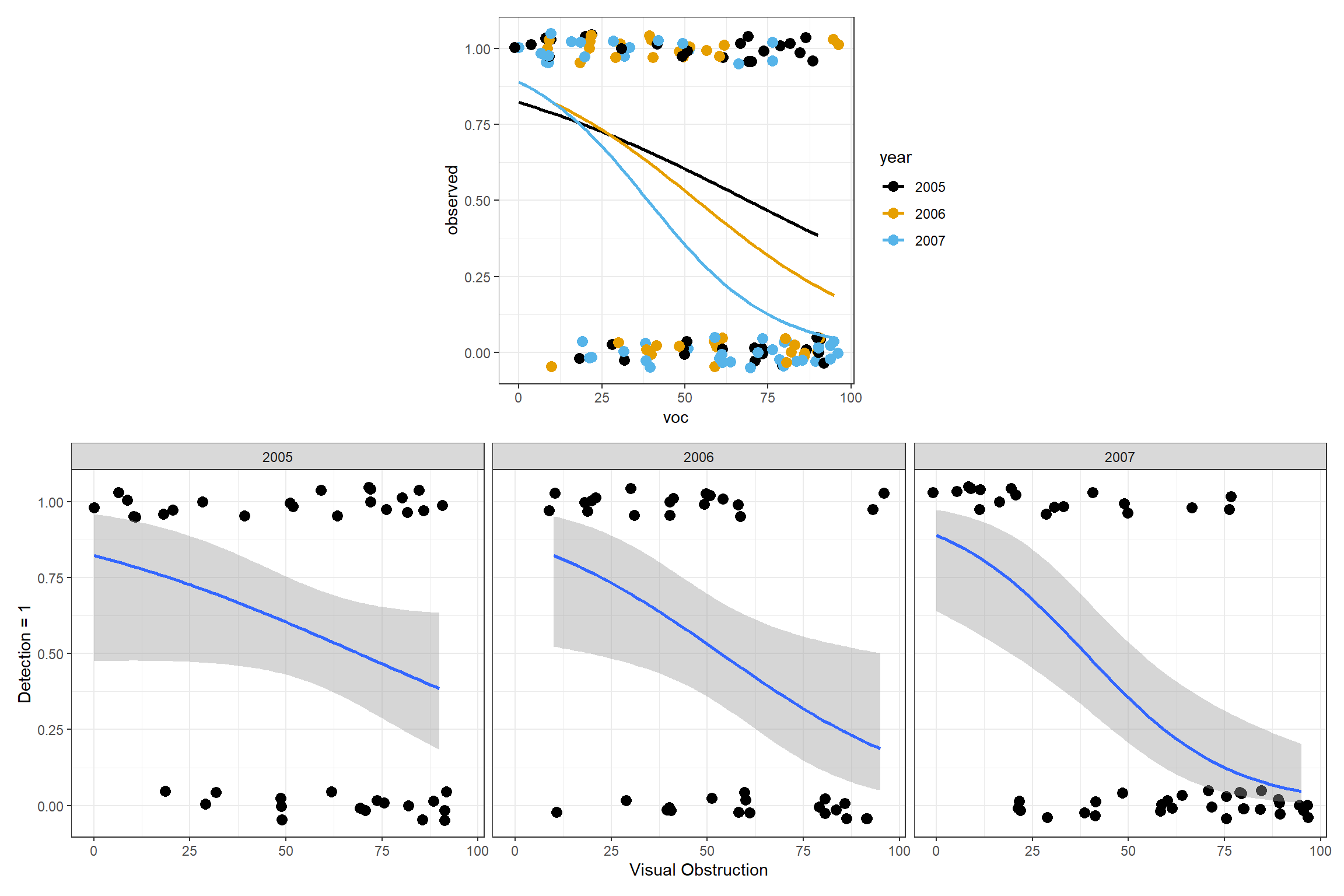
FIGURE 16.7: Fitted logistic regression model relating detection probabilities to the amount of visual obstruction, year, and their interaction.
What if we fit more complicated models containing multiple predictor variables? We have a few options:
- We can create predicted values for different combinations of our explanatory variables, their standard errors, and then plot the results.
- We can use one or more R packages to automate this process. In Section 16.5.4, we will explore the
effects(Fox & Weisberg, 2018) andggeffectspackages (Lüdecke, 2018), which were also introduced in Section 3.13 when we discussed creating partial residual plots.
Let’s begin by creating our own plots, which will give us insights into how these latter packages work.
16.5.1 Predictions and confidence intervals
Let’s begin by considering our initial model containing only voc. We can summarize models in terms of: \(\hat{E}[Y_i|X_i] = \hat{p}_i= \hat{P}(Y_i=1 | voc_i)\) for a range of voc values. The easiest way to accomplish this is to use the predict function in R. Specifically, we can generate predictions for a range of values of voc using:
voc.p<-seq(1, 99, length = 100)
p.hat <- predict(mod1, newdata = data.frame(voc = voc.p), type = "response")
plot(voc.p, p.hat, xlab = "VOC", ylab = "Pr(detect | voc)", type = "l")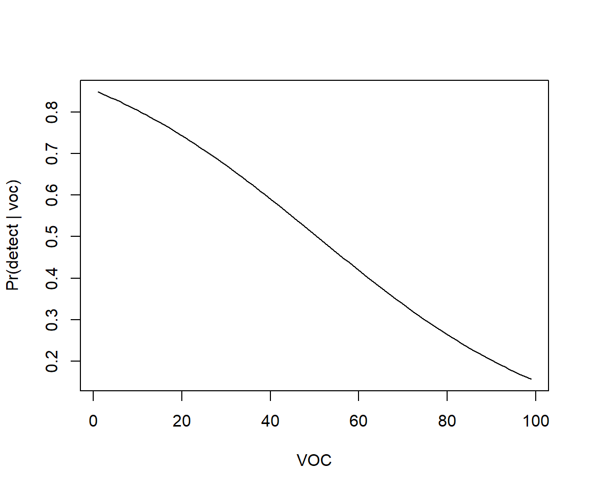
FIGURE 16.8: Predicted probability of detection as a function of visual obstruction (voc).
We could also ask the predict function to return standard errors associated with our predictions by adding the argument se.fit=TRUE. If we ask for SEs on the response scale, these standard errors will be calculated using the delta method (see Section 10.7.1). We could then use \(\hat{p}_i\pm 1.96SE\) to form confidence intervals for our plot, depicting how \(p_i\) (and our uncertainty about \(p_i\)) depends on voc. Remember, that \(p_i\) has to be between 0 and 1, and there is no guarantee that these confidence intervals will remain \(\le 1\) or \(\ge 0\). A better approach is to use predict to generate estimates on the link (i.e., logit) scale, along with standard errors on this scale. Using this information, we can then form a confidence interval for \(\text{logit}(p_i)\) and then back-transform this interval using the plogis function to get a confidence interval for \(p_i\). This approach has several advantages:
The sampling distribution for \(\text{logit}(\hat{p}_i) = \hat{\beta}_0 + \hat{\beta}_1X_{1,i} + \ldots \hat{\beta}_pX_{p,i}\) tends to be more “Normal” than the sampling distribution for \(\hat{p}_i\).
Confidence intervals will be guaranteed to live on the (0,1) scale. Also, note that the intervals will not be symmetric.
The code and plot below compares these two approaches:
# Predictions response scale
newdat <- data.frame(voc = seq(1, 99, length = 100))
phat <- predict(mod1, type = "resp", se.fit = T,newdata = newdat)
lcl.r <- phat$fit + 1.96 * phat$se.fit
ucl.r <- phat$fit - 1.96 * phat$se.fit

# Predictions link scale
phat2<-predict(mod1, type = "link", se.fit = T, newdata = newdat)
lcl.l <- plogis(phat2$fit + 1.96 * phat2$se.fit)
ucl.l <- plogis(phat2$fit - 1.96 * phat2$se.fit)
pe.l <- plogis(phat2$fit)

# Combine and plot
newdat <- cbind(newdat, phat = phat$fit, lcl.r, ucl.r, phat2 = phat2$fit, lcl.l, ucl.l, pe.l)
ggplot(newdat, aes(voc, phat)) + geom_line() +
  geom_line(aes(voc, lcl.l), lty = 2, col = "blue") +
  geom_line(aes(voc, ucl.l), lty = 2, col = "blue") +
  geom_line(aes(voc, lcl.r), lty = 2, col = "red") +
  geom_line(aes(voc, ucl.r), lty = 2, col = "red") +
  xlab("Visual Obstruction") + ylab(expression(hat(p)))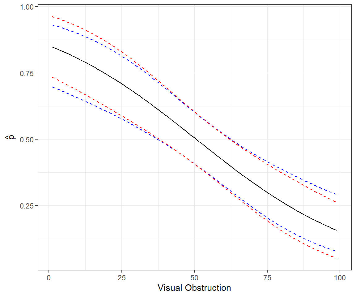
FIGURE 16.9: Comparison of methods for forming confidence intervals on the response scale in red versus link scale with back transformation in blue.
16.5.2 Aside: Revisiting predictions using matrix algebra
How does R and the predict function work? Here, we briefly revisit the ideas from Sections 5.4 and 3.11. Remember, glm estimates \(\beta\) using Maximum Likelihood, specifically, by maximizing:
\[L(\beta; y, x) = \prod_{i=1}^{n}p_i^{y_i}(1-p_i)^{1-y_i} \mbox{ with}\]
\[p_i = \frac{e^{\beta_0 + \beta_1X_{1 ,i}+ \ldots \beta_pX_{p,i}}}{1+e^{\beta_0 + \beta_1X_{1,i} + \ldots \beta_pX_{p,i}}}\]
Also, remember, for large samples, \(\hat{\beta} \sim N(\beta, I^{-1}(\beta))\). We can use this theory to conduct hypothesis tests (see the p-values using z-statistics in the output by the summary function) and to get confidence intervals.
Let \(X\) = be our design matrix, in this case consisting of 2 columns (a column of 1’s for the intercept and a second column containing the voc measurements). Again, we can use model.matrix to see what this design matrix looks like.
Let \(\beta = (\beta_0, \beta_1)\), our vector of parameters (intercept and slope).
We can calculate \(\text{logit}(\hat{p}_i|X_i)\) and its SE using matrix multiplication:
- \(\text{logit}(\hat{p}_i|X_i) = X\hat{\beta}\) (use
%*%in R to perform matrix multiplication) - Variance/covariance of \(\text{logit}(\hat{p}|X) = X(\hat{I}^{-1}(\beta))X^T\) (we access our estimate of \(I^{-1}(\beta)\) using
vcov(mod1)).
The code below demonstrates that we get the same results using matrix multiplication as when using the predict function.
newdata <- data.frame(observed = 1, voc = voc.p)
xmat <- model.matrix(mod1, data = newdata)
p.hat.check <- xmat %*% coef(mod1)
p.se.check <- sqrt(diag(xmat %*% vcov(mod1) %*% t(xmat)))
# Compare predictions
summary(predict(mod1, newdata = newdata, type = "link") - p.hat.check)
## V1
## Min. :0
## 1st Qu.:0
## Median :0
## Mean :0
## 3rd Qu.:0
## Max. :0# Compare SEs
summary(predict(mod1, newdata = newdata, type = "link", se.fit = TRUE)$se.fit - p.se.check)## Min. 1st Qu. Median Mean 3rd Qu. Max.
## -1.110e-16 -2.776e-17 0.000e+00 -3.886e-18 0.000e+00 1.110e-1616.5.3 Additive effects on logit scale \(\ne\) additive effects on probability scale
Creating an interpreting effect plots is a little trickier than it might seem due to modeling the mean on the logit scale. Let’s consider our second model:
\[Y_i|X_i \sim \text{Bernoulli}(p_i)\] \[\text{logit}(p_i) = \beta_0 + \beta_1voc_i + \beta_2I(year=2006)_i+\beta_3I(year=2007)_i\]
Here, the effects of year and voc are “additive” on the logit scale, and thus, differences in logit(\(p_i\)) between years do not depend on voc. However, the effects of voc and year are multiplicative on the odds scale and even more complicated on the \(p\) scale (see e.g., the discussion related to parameter interpretation in Section 16.2). As a result, differences in \(p_i\) between years will depend on voc and the effect of voc on \(p\) will depend on the year (even though we do not have an interaction in the model!).
To see this in action, let’s plot \(\text{logit}(p_i)\) and \(p_i\) versus voc for the different years (Figure 16.10). Note that distances between the lines for the different years are constant when we look at \(\text{logit}(p_i)\) but not when we plot \(p_i\) (the curves are closer together as \(p_i\) approaches 0 or 1). These differences result from having to back-transform from the logit to response scale.
  newdat<-expand.grid(voc=seq(0,100,5), year=unique(exp.m$year))
  newdat$p.hats<-predict(mod2, newdat=newdat, type="response")
  newdat$logit.p.hats<-predict(mod2, newdata=newdat, type="link")
  plot.logitp<-ggplot(newdat, aes(voc, logit.p.hats, colour=year))+geom_line()+
    ylab("logit(p)")
  plot.p<-ggplot(newdat, aes(voc, p.hats, colour=year))+geom_line()+ylab("p")
plot.logitp + plot.p 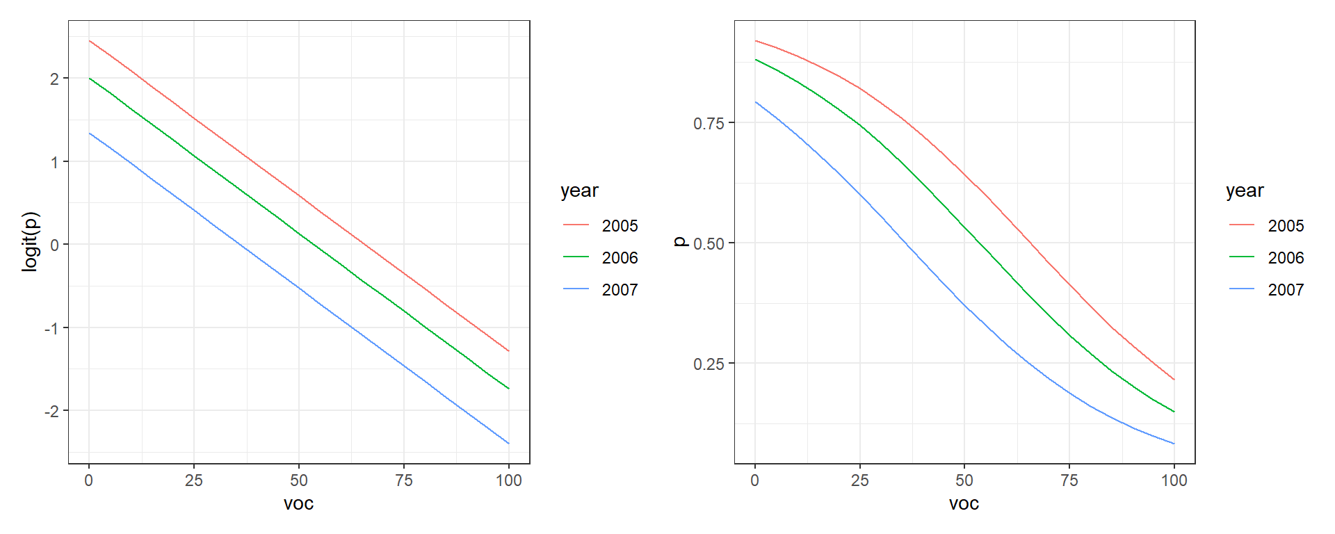
FIGURE 16.10: Relationships between the amount of visual obstruction (voc) and logit(p) and p.
16.5.4 Effect plots for complex models: Using the effects and ggpredict packages
Recall from Section 3.13.3, we can visualize the effect of predictors using effect plots formed by varying 1 predictor while holding all other predictors at a common value (e.g., the mean for continuous variables and the modal value for categorical variables). The expand.grid function, used in the creation of Figure 16.10 can be a big help here as it makes it easy to create a data set containing all combinations of multiple predictor variables. Still, creating effect plots from scratch can be a little tedious. The effects and ggeffects packages can makes this process a little easier.
16.5.4.1 Effects package
The effect function in the effects` package:
- Fixes all continuous variables (other than the one of interest) at their mean values
- For categorical predictors, it averages predictions on the link scale, weighted by the proportion of observations in each category
By default, plots are constructed on the link scale, but we can add type="response" to create a plot on response scale. Examples are given in Figures 16.11, 16.12, and 16.13.
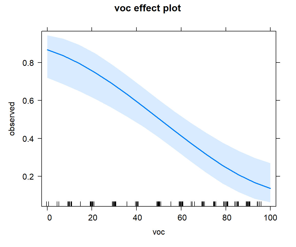
FIGURE 16.11: Effect plot showing how the probability of detection varies with voc.
We can add partial residuals using adding parital.residuals = TRUE to the `effect function (Figure 16.12). For binary data, it is difficult to interpret the raw residuals, but this option also overlays a smooth line capturing any trend.
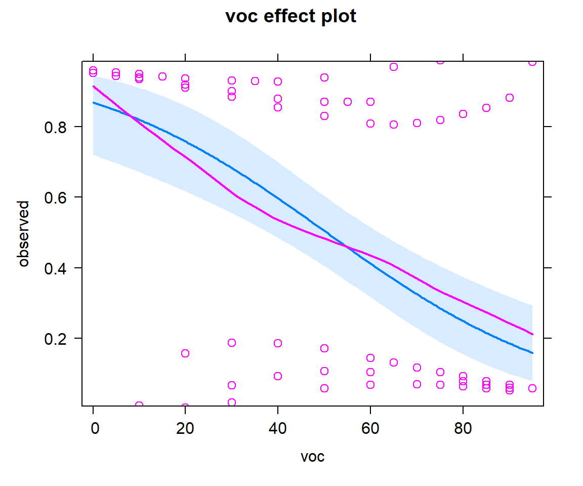
FIGURE 16.12: Effect plot with partial residuals added, showing how the probability of detection varies with voc
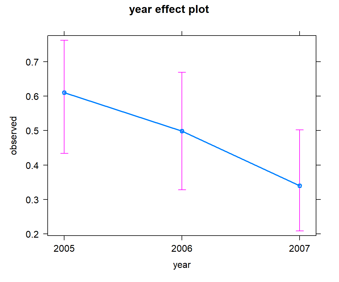
FIGURE 16.13: Effect plot showing how the probability of detection varied across years.
We can also use effect and the summary functions to return numerical values (estimates and confidence intervals):
 year effect
year
     2005      2006      2007
0.6105102 0.4988990 0.3401946

 Lower 95 Percent Confidence Limits
year
     2005      2006      2007
0.4338786 0.3283351 0.2086299

 Upper 95 Percent Confidence Limits
year
     2005      2006      2007
0.7622325 0.6697194 0.5020875
Alternatively, we can use the ggeffect function in the ggeffects package to format the output as a list with an associated print function.
## $voc
## # Predicted probabilities of observed
##
## voc | Predicted |       95% CI
## ------------------------------
##   0 |      0.87 | [0.72, 0.94]
##  10 |      0.82 | [0.67, 0.91]
##  20 |      0.76 | [0.62, 0.86]
##  35 |      0.64 | [0.52, 0.74]
##  55 |      0.46 | [0.36, 0.56]
##  65 |      0.37 | [0.27, 0.47]
##  75 |      0.29 | [0.19, 0.41]
##  95 |      0.16 | [0.08, 0.29]
##
## $year
## # Predicted probabilities of observed
##
## year | Predicted |       95% CI
## -------------------------------
## 2005 |      0.61 | [0.43, 0.76]
## 2006 |      0.50 | [0.33, 0.67]
## 2007 |      0.34 | [0.21, 0.50]
##
## attr(,"class")
## [1] "ggalleffects" "list"
## attr(,"model.name")
## [1] "mod2"
There is also a plot function that we can use with the ggeffect function to visualize these effects (Figure 16.14).
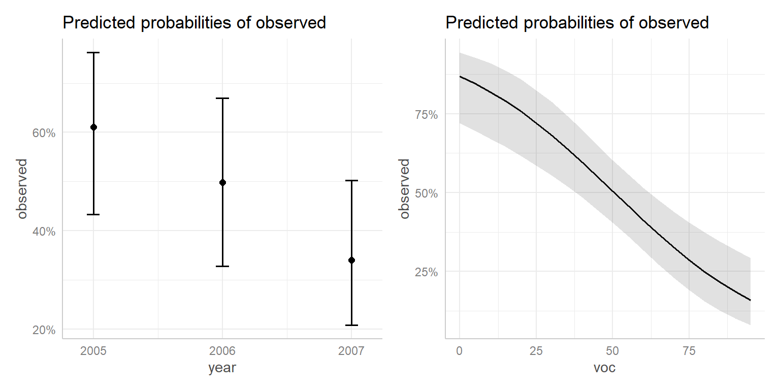
FIGURE 16.14: Effect plot created using the ggeffects package.
Or, we can specify specific terms for which we want estimates. In this case, ggeffects will return a data.frame from which we can create our own plot using ggplot (Figure 16.15).
effects.mod2 <- ggeffect(mod2, terms = c("voc", "year"))
ggplot(effects.mod2, aes(x, predicted, col = group)) + geom_line()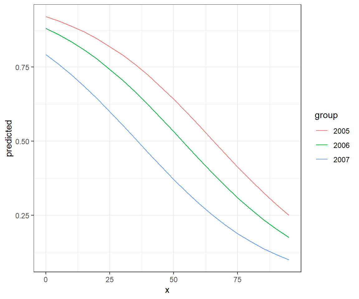
FIGURE 16.15: Effect plot created using the ggeffects package along with ggplot.
And again, we could add partial residuals and a smooth line to our plot (Figure 16.16).
## `geom_smooth()` using formula 'y ~ x'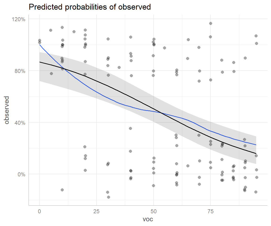
FIGURE 16.16: Effect plot created using the ggeffects package with partial residuals overlayed.
16.5.5 Understanding effect estimates from the effects and ggeffects package
The goal of this section is to illuminate how the estimates and confidence intervals on the response scale are formed when using the effects package or the ggeffects function in the ggeffects package. Lets start by considering the effects for the different years. These are formed by setting voc at its mean value, and estimating:
\(P(Y_i = 1 | year = year_i, voc = \overline{voc})\) for each of the years in the data set. These estimates are easy to understand and recreate using the predict function:
newdata<-data.frame(voc = rep(mean(exp.m$voc), 3),
                    year = c("2005", "2006", "2007"))
predict(mod2, newdata = newdata, type = "resp")
1 2 3
0.6105102 0.4988990 0.3401946
 year effect
year
     2005      2006      2007
0.6105102 0.4988990 0.3401946
Now, how does the effects package estimate the effect of voc? There is no “mean or average” year since year is a categorical variable. Instead, it calculates a weighted mean of the predictions for each year on the link scale, with weights given by the proportion of observations in each category. It then back-transforms this weighted mean.
 voc effect
voc
        0        20        50        70       100
0.8684553 0.7575962 0.5044524 0.3251918 0.1356677
# Proportion of observations in each year (will be used to form weights)
weights <- data.frame(table(exp.m$year) / nrow(exp.m))
names(weights) = c("year", "weight")
weights year weight
1 2005 0.3145161
2 2006 0.2983871
3 2007 0.3870968# New data for predictions
newdata <- data.frame(expand.grid(year = c("2005", "2006", "2007"),
voc = seq(0, 100, 20)))
newdata <- left_join(newdata, weights)
# Predictions on link scale
newdata$logit.phat <- predict(mod2, newdata = newdata, type = "link")
# Weight predictions and backtransform
newdata %>% group_by(voc) %>% dplyr::summarize(plogis(sum(logit.phat * weight)))# A tibble: 6 x 2
voc `plogis(sum(logit.phat * weight))`
<dbl> <dbl>
1 0 0.868
2 20 0.758
3 40 0.597
4 60 0.412
5 80 0.249
6 100 0.13616.5.6 Predictions using the ggpredict function
Whereas the effects function averages predictions across the different levels of a categorical predictor, producing what are sometimes referred to as marginal effects, the ggpredict function will provide adjusted predictions where all variables except a focal variable remain fixed at their mean, modal, or user-specified values. We first demonstrate this approach for our additive model with voc and year.
## $voc
## # Predicted probabilities of observed
##
## voc | Predicted |       95% CI
## ------------------------------
##   0 |      0.92 | [0.77, 0.98]
##  10 |      0.89 | [0.73, 0.96]
##  20 |      0.85 | [0.67, 0.94]
##  35 |      0.76 | [0.58, 0.88]
##  55 |      0.60 | [0.42, 0.75]
##  65 |      0.51 | [0.34, 0.67]
##  75 |      0.41 | [0.25, 0.59]
##  95 |      0.25 | [0.12, 0.45]
##
## Adjusted for:
## * year = 2005
##
## $year
## # Predicted probabilities of observed
##
## year | Predicted |       95% CI
## -------------------------------
## 2005 |      0.55 | [0.38, 0.71]
## 2006 |      0.44 | [0.28, 0.62]
## 2007 |      0.29 | [0.17, 0.45]
##
## Adjusted for:
## * voc = 60.00
##
## attr(,"class")
## [1] "ggalleffects" "list"
## attr(,"model.name")
## [1] "mod2"
As with the ggeffects function, if we specify terms from the model, the function will return a data.frame that can be easily plotted.
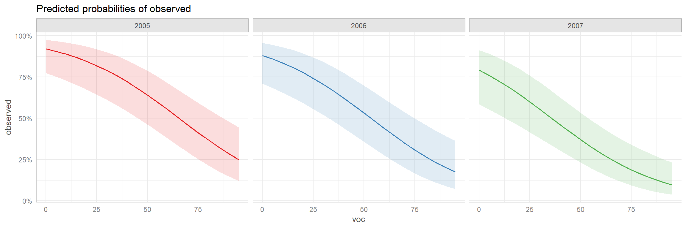
FIGURE 16.17: Adjusted prediction plot created using the ggeffects package.
This approach can be particularly useful when there are interactions between variables as in our mod3 (Figure 16.18).
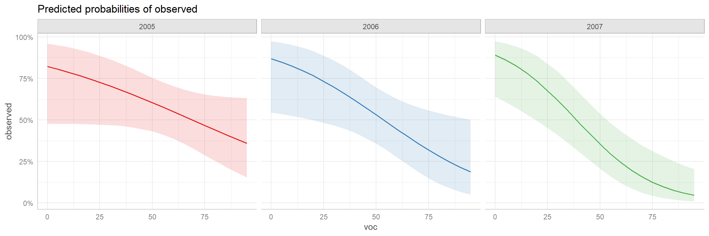
FIGURE 16.18: Adjusted prediction plot for the interaction model created using the ggeffects package.
16.6 Logistic regression: Bayesian implementations
Again, an advantage of implementing models in JAGS is that we will be forced to be very clear about the model we are fitting. Specifically, we will have to write down the likelihood with the expression relating \(\text{logit}(p)\) to our predictor variables. Contrast this process with fitting a model using glm where users may not even know that the mean is being modeled on a transformed scale.
In this section, we will fit the logistic regression model containing only voc, leaving the model with year and voc as an in-class exercise. Before we look at JAGS code for fitting this model, it is helpful to give some thought to priors for our regression parameters. It turns out that specifying priors can be a bit tricky. We can specify priors that are vague (meaning they take on a wide range of values, all equally likely) on the logit scale, but this may then imply something very specific when viewed on the \(p\) scale. Consider, for example, the model below, where \(p\) is constant and we specify our prior on the logit scale:
\[Y_i \sim \text{Bernoulli}(p)\] \[\text{logit}(p) = \beta_0\] \[\beta_0 \sim N(0,10^2)\]
It turns out (see Fig. 16.19) that this prior is not at all vague when viewed on the \(p\) scale. In particular, this prior suggests that \(p\) is extremely likely to be very near 0 or 1 and unlikely to take on any value in between these two extremes.
par(mfrow=c(1,2))
beta0<-rnorm(10000,0,100)
p<-plogis(beta0)
hist(beta0, xlab=expression(beta[0]),
     main=expression(paste("Prior distribution for ", beta[0])),
     col="gray")
hist(p, xlab="p", main="Prior distribution for p", col="gray")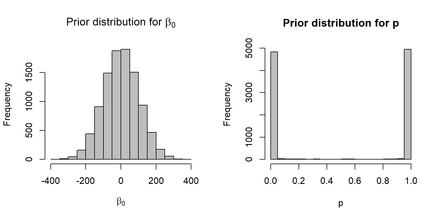
FIGURE 16.19: A N(0,100) prior distribution for logit(p) results in a non-vague prior on the p scale.
If the goal is to achieve a near uniform distribution for \(p\), it turns out that a \(N(0, 3)\) distribution is a much better option (Fig. 16.20):
par(mfrow=c(1,2))
beta0<-rnorm(10000, 0, sqrt(3))
p<-plogis(beta0)
hist(beta0, xlab=expression(beta[0]),
     main=expression(paste("Prior distribution for ", beta[0])),
     col="gray")
hist(p, xlab="p", main="Prior distribution for p", col="gray")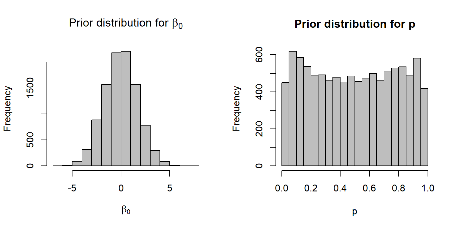
FIGURE 16.20: A \(N(0, \sqrt{3})\) distribution for the prior on the logit scale, resulting in a near uniform prior distribution on the \(p\) scale.
Establishing recommendations for default priors is a high priority and active research area within the Bayesian community (see discussion here: https://github.com/stan-dev/stan/wiki/Prior-Choice-Recommendations). For logistic regression models, Gelman, Jakulin, Pittau, Su, & others (2008) recommended:
- Scaling continuous predictors so they have mean 0 and sd = 0.5.
- Using a Cauchy prior, with precision parameter = \(\frac{1}{2.5^2}= 0.16\); this distribution is equivalent to a Student-t distribution with 1 degree of freedom and can be specified in JAGS as:
dt(0, pow(2.5,-2), 1).
Both \(t-\) and Normal distributions assume most effect sizes are near 0, but the \(t-\)distribution allows for the possibility of more extreme values since a t-distribution has wider tails than a Normal distribution (Figure 16.21)54.
library(LaplacesDemon)
curve(dnorm(x, mean=0, sd=2.5), from=-8, to=8, ylab="Density")
curve(dstp(x, mu=0, tau=1/2.5^2, n=1), from=-8, to=8, add=TRUE, lty=2)
legend(2, 0.15, c("Normal", "t"), lty=c(1,2), bty="n")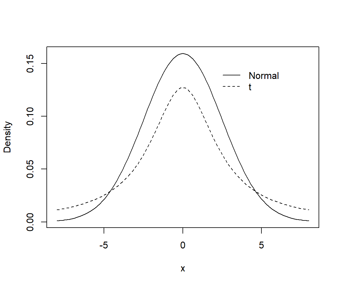
FIGURE 16.21: Comparison of Normal (solid curve) and Student-t prior (dashed curve) for logistic regression models.
In general, we may seek a non-informative prior, which means that we want our answers to be determined primarily by the data and likelihood and not the prior. On the other hand, an advantage of a Bayesian approach is that we can potentially take advantage of previous knowledge and data when this information exists and we want it to influence our results. I.e., there may be times when using an informative prior can be beneficial. Further, many would argue for weakly informative priors that “regularize” or shrink parameters towards 0 [e.g., McElreath (2020)). This approach is often used to improve predictive performance, particularly in cases where one is faced with having too many explanatory variables relative to one’s sample size (Section 8.6).
16.6.1 Fitting the logistic regression model to moose data
Below, we use Gelman’s suggested prior when analyzing the moose data in JAGS:
lrmod<-function(){

  # Priors
  # Note: Gelman recommends
  # - scaling continuous predictors so they have mean 0 and sd = 0.5
  # - using a non-informative Cauchy prior dt(0, pow(2.5,-2), 1)
  # see arxiv.org/pdf/0901.4011.pdf
  alpha ~ dt(0, pow(2.5, -2), 1)
  beta ~ dt(0, pow(2.5, -2), 1)

  # Likelihood
  for(i in 1:n){
    logitp[i] <- alpha + beta * voc[i]
    p[i] <- exp(logitp[i]) / (1 + exp(logitp[i]))
    observed[i] ~ dbin(p[i], 1)

    # GOF test
    presi[i] <- (observed[i] - p[i]) / sqrt(p[i] * (1 - p[i]))
    obs.new[i] ~ dbin(p[i], 1)
    presi.new[i] <- (obs.new[i] - p[i]) / sqrt(p[i] * (1 - p[i]))
    D[i] <- pow(presi[i], 2)
    D.new[i] <- pow(presi.new[i], 2)
  }
  fit <- sum(D[])
  fit.new <- sum(D.new[])
}


# Bundle data
voc <- (exp.m$voc - mean(exp.m$voc)) / (0.5 * sd(exp.m$voc))
jagsdata <- list(observed = exp.m$observed, voc = voc, n = nrow(exp.m))


# Parameters to estimate
params <- c("alpha", "beta", "p", "presi", "fit", "fit.new")

# MCMC settings
nc <- 3
ni <- 3000
nb <- 1000
nt <- 2

out.p <- jags.parallel(data = jagsdata, parameters.to.save = params,
                      model.file = lrmod, n.thin= 2, n.chains = 3,
                      n.burnin = 1000, n.iter = 3000)

#Goodness-of-fit test
fitstats <- MCMCpstr(out.p, params = c("fit", "fit.new"), type = "chains")
T.extreme <- fitstats$fit.new >= fitstats$fit
(p.val <- mean(T.extreme))
## [1] 0.4643333Looking at the goodness-of-fit test (above), we again fail to reject the null hypothesis that our model is appropriate for the data. Below, we compare estimates of coefficients and 95% credible intervals to estimates and CI from fitting the same model (using the scaled data) via glm:
##         mean    sd   2.5%    50%  97.5% Rhat n.eff
## alpha -0.101 0.197 -0.494 -0.099  0.277    1  2730
## beta  -0.497 0.112 -0.738 -0.494 -0.280    1  2759
mod1b <- glm(exp.m$observed ~ scale(voc), family = binomial(),
data = exp.m)
cbind(coef(mod1b), confint(mod1b))## Waiting for profiling to be done...## 2.5 % 97.5 %
## (Intercept) -0.1045001 -0.4980208 0.2864257
## scale(voc) -0.9741428 -1.4229581 -0.5670762What if we had naively used extremely vague priors for our regression parameters? We can compare the results, below, using the MCMCplot function in the MCMCvis package:
lrmodv<-function(){

  alpha~dnorm(0, 0.0001)
  beta~dnorm(0, 0.0001)

  # Likelihood
  for(i in 1:n){
    logitp[i]<-alpha+beta*voc[i]
    p[i]<-exp(logitp[i])/(1+exp(logitp[i]))
    observed[i]~dbin(p[i],1)
  }
}

params <- c("alpha", "beta")
out.p.vague <- jags.parallel(data = jagsdata, parameters.to.save = params,
                             model.file = lrmodv, n.thin= 2, n.chains = 3,
                             n.burnin = 1000, n.iter = 3000)

MCMCplot(object = out.p, object2=out.p.vague, params=c("alpha", "beta"),
         offset=0.1, main='Posterior Distributions')
In this case, the priors make little difference to our end results, but that may not always be the case.
16.7 Aside: logistic regression with multiple trials
If we have multiple observations for each unique set of predictor variables, then we can write the model as:
\[Y_i | X_i \sim Binomial(n_i, p_i)\]
\[logit(p_i) = \log\left(\frac{p_i}{1-p_i}\right) = \beta_0 + \beta_1X_{1,i}+\ldots \beta_kX_{k,i}\]
This formulation can provide significant increases in speed when fitting large data sets (see e.g., Iannarilli, Arnold, Erb, & Fieberg, 2019). The glm function allows us to fit a logistic regression model to data containing the number of trials and the number of successes. We will demonstrate the approach using a famous data set from Bliss (1935), which contains the number of adult flour beetles killed after 5 hours of exposure to gaseous carbon disulfide at various concentrations. The data are contained in a number of different R packages, including the glmx package. We access the data using:
## Warning: package 'glmx' was built under R version 4.1.3## dose died n
## 1 1.6907 6 59
## 2 1.7242 13 60
## 3 1.7552 18 62
## 4 1.7842 28 56
## 5 1.8113 52 63
## 6 1.8369 53 59
## 7 1.8610 61 62
## 8 1.8839 60 60Let \(Y_i\) be the number of individuals that died and \(n\) be the number of beetles exposed to each dosage level. We will assume:
\[Y_i | Dosage_i \sim Binomial(n_i, p_i)\]
\[logit(p_i) = \log\left(\frac{p_i}{1-p_i}\right) = \beta_0 + \beta_1 Dosage_i\]
We can fit the model using:
lrdose <- glm(cbind(died, n - died) ~ dose, data = BeetleMortality, family = binomial())
summary(lrdose)
##
## Call:
## glm(formula = cbind(died, n - died) ~ dose, family = binomial(),
## data = BeetleMortality)
##
## Deviance Residuals:
## Min 1Q Median 3Q Max
## -1.5941 -0.3944 0.8329 1.2592 1.5940
##
## Coefficients:
## Estimate Std. Error z value Pr(>|z|)
## (Intercept) -60.717 5.181 -11.72 <2e-16 ***
## dose 34.270 2.912 11.77 <2e-16 ***
## ---
## Signif. codes: 0 '***' 0.001 '**' 0.01 '*' 0.05 '.' 0.1 ' ' 1
##
## (Dispersion parameter for binomial family taken to be 1)
##
## Null deviance: 284.202 on 7 degrees of freedom
## Residual deviance: 11.232 on 6 degrees of freedom
## AIC: 41.43
##
## Number of Fisher Scoring iterations: 4To demonstrate that we get the same result if we fit a model to data containing a separate record for each observation, we create a “long format” data set below:
BeetleLong <- NULL
uid <- unique(BeetleMortality$dose)
for(i in seq_along(uid)){
  tempdat <- BeetleMortality[i,]
  BeetleLong <- rbind(BeetleLong,
                      data.frame(died = c(rep(1, tempdat$died), rep(0, tempdat$n- tempdat$died)),
                                 dose = rep(tempdat$dose, tempdat$n)))
}
head(BeetleLong)
## died dose
## 1 1 1.6907
## 2 1 1.6907
## 3 1 1.6907
## 4 1 1.6907
## 5 1 1.6907
## 6 1 1.6907## # A tibble: 8 x 3
## dose died trials
## <dbl> <dbl> <int>
## 1 1.69 6 59
## 2 1.72 13 60
## 3 1.76 18 62
## 4 1.78 28 56
## 5 1.81 52 63
## 6 1.84 53 59
## 7 1.86 61 62
## 8 1.88 60 60We then fit the same regression model to the set of Bernoulli trials showing that we get the same result:
##
## Call:
## glm(formula = died ~ dose, family = binomial(), data = BeetleLong)
##
## Deviance Residuals:
##     Min       1Q   Median       3Q      Max
## -2.4922  -0.5986   0.2058   0.4512   2.3820
##
## Coefficients:
##             Estimate Std. Error z value Pr(>|z|)
## (Intercept)  -60.717      5.181  -11.72   <2e-16 ***
## dose          34.270      2.912   11.77   <2e-16 ***
## ---
## Signif. codes:  0 '***' 0.001 '**' 0.01 '*' 0.05 '.' 0.1 ' ' 1
##
## (Dispersion parameter for binomial family taken to be 1)
##
##     Null deviance: 645.44  on 480  degrees of freedom
## Residual deviance: 372.47  on 479  degrees of freedom
## AIC: 376.47
##
## Number of Fisher Scoring iterations: 5
16.8 Aside: Complete Separation
Occasionally, when fitting a logistic regression model, you may encounter a warning message that the glm fitting algorithm “did not converge” or that “fitted probabilities numerically 0 or 1 occurred.” This is indicative of a problem referred to as complete separation – in which a predictor variable or set of predictor variables is able to separate a response variable into separate classifications of 0’s and 1’s.
To demonstrate, we will use an example developed by Jack Weiss using data from Piegorsch & Bailer (2005) collected to evaluate water quality and potential contamination by an industrial solvent trichloroethylene (TCE). The data are included in the Data4Ecologists package and can be accessed using:
We will build a logistic regression model to describe the probability that a well will be contaminated with TCE as a function of the surrounding land use category (land.use) and whether or not sewers were used in the area surrounding the well (sewer). The data set is formatted so that each observation has a unique set of covariates, with y quantifying the number of wells contaminated with TSE and n . Thus, we model the data using glm with a cbind(successes, failures) syntax as described in Section 16.7:
##
## Call:
## glm(formula = cbind(y, n - y) ~ land.use + sewer, family = binomial(),
##     data = wells)
##
## Deviance Residuals:
##     Min       1Q   Median       3Q      Max
## -1.5364  -0.9860  -0.0002   0.3542   1.4394
##
## Coefficients:
##                Estimate Std. Error z value Pr(>|z|)
## (Intercept)     -3.6568     0.7376  -4.957 7.14e-07 ***
## land.usecomm     1.8676     0.8044   2.322  0.02025 *
## land.useindus    2.2070     0.8053   2.741  0.00613 **
## land.useinst     0.7584     0.8395   0.903  0.36629
## land.userecr     0.6676     0.8435   0.791  0.42870
## land.useresH     1.7316     0.7784   2.225  0.02611 *
## land.useresL     0.6663     1.0501   0.635  0.52572
## land.useresM     1.0212     0.7809   1.308  0.19099
## land.usetrans    0.7933     0.8360   0.949  0.34267
## land.useundev  -18.3414  3033.9308  -0.006  0.99518
## seweryes         1.5980     0.2955   5.407 6.41e-08 ***
## ---
## Signif. codes:  0 '***' 0.001 '**' 0.01 '*' 0.05 '.' 0.1 ' ' 1
##
## (Dispersion parameter for binomial family taken to be 1)
##
##     Null deviance: 146.956  on 19  degrees of freedom
## Residual deviance:  15.201  on  9  degrees of freedom
## AIC: 82.476
##
## Number of Fisher Scoring iterations: 17
Although we didn’t receive a warning in this case, inspecting the model coefficients and their SEs we see the symptoms of complete separation - namely a coefficient for land.useundev that is extreme and an associated SE that is also large.
Think-Pair-Share: Estimate the probability that a well placed in undeveloped land without sewers has TSE contamination. What do you think this indicates about the underlying data?
We can estimate the probability that a well placed in undeveloped land has TSE contamination by adding the intercept and the coefficient for land.useundev and then taking the inverse logit transformation:
##  (Intercept)
## 2.794265e-10
We see that this probability is extremely small. Let’s look at the observations broken down by land use category:
wells %>% mutate(nocontam = n-y) %>% group_by(land.use) %>%
  dplyr::summarize(contam = sum(y), noncontam = sum(nocontam))
## # A tibble: 10 x 3
## land.use contam noncontam
## <chr> <int> <int>
## 1 agri 2 53
## 2 comm 20 29
## 3 indus 20 25
## 4 inst 8 46
## 5 recr 7 57
## 6 resH 34 59
## 7 resL 2 24
## 8 resM 17 112
## 9 trans 8 51
## 10 undev 0 76We see that there are no wells in undeveloped areas that were contaminated. Thus, the smaller the coefficient for land.useundev the better – essentially, the numerical optimizer keeps moving towards \(\infty\) but at some point the likelihood becomes extremely flat (e.g., consider that our current estimate already equates to a probability on the order fo \(1^{-10}\)). Also, recall that flat likelihoods result in large SEs when estimated using the Hessian (see Section 10.5).
There are several different approaches that we might use to deal with this problem. One simple solution would be to group land use categories so that we no longer have complete separation. Another popular approach is to use penalized likelihood or Bayesian approaches (Firth, 1993; Fijorek & Sokolowski, 2012). Let’s consider a Bayesian model with \(N(\mu = 0, \sigma^2 = 3)\) priors:
lrmod<-function(){

  # Priors
  for(i in 1:nlanduse){
    beta.landuse[i] ~ dnorm(0, 1/3)
  }
  beta.sewer ~ dnorm(0, 1/3)
  # Likelihood
  for(i in 1:nobs){
    logit(p[i]) <-beta.landuse[landuse[i]] + beta.sewer * sewer[i]
    y[i]~dbin(p[i], n[i])
  }
}


# Bundle data
jags.data <- list(y = wells$y,
                  landuse = as.numeric(as.factor(wells$land.use)),
                  sewer = as.numeric(as.factor(wells$sewer)),
                  n = wells$n, nobs = nrow(wells),
                  nlanduse = length(unique(wells$land.use)))


# Parameters to estimate
params <- c("beta.landuse", "beta.sewer")

# MCMC settings
nc <- 3
ni <- 3000
nb <- 1000
nt <- 2

lr.bayes <- jags.parallel(data = jags.data, parameters.to.save = params,
                       model.file = lrmod, n.thin = 1, n.chains = 3,
                       n.burnin = 1000, n.iter = 5000)
Let’s look to make sure everything converged and inspect the SE’s of the different coefficients:
##                       mean         sd       2.5%        50%       97.5% Rhat
## beta.landuse[1]  -3.587814  0.6073940 -4.8247411 -3.5604594  -2.4832725 1.02
## beta.landuse[2]  -1.463457  0.4863417 -2.4085845 -1.4653444  -0.5082888 1.00
## beta.landuse[3]  -1.231906  0.4713098 -2.1471992 -1.2345322  -0.3064563 1.00
## beta.landuse[4]  -2.656346  0.4941036 -3.6411895 -2.6549084  -1.6979328 1.01
## beta.landuse[5]  -2.891551  0.4991950 -3.9187910 -2.8830222  -1.9718231 1.01
## beta.landuse[6]  -1.637646  0.4333541 -2.4760085 -1.6414424  -0.7911272 1.00
## beta.landuse[7]  -2.936314  0.6705834 -4.3194755 -2.8966989  -1.7119706 1.01
## beta.landuse[8]  -2.688568  0.3981482 -3.4558552 -2.6962779  -1.9153455 1.01
## beta.landuse[9]  -2.672110  0.4940992 -3.6768105 -2.6688090  -1.7112487 1.00
## beta.landuse[10] -4.726058  0.7601821 -6.3112348 -4.6971673  -3.3747042 1.02
## beta.sewer        0.599020  0.2092529  0.1864398  0.6002753   0.9993316 1.00
## deviance         87.062768 10.8333724 73.9455898 86.1707714 103.4192716 1.00
##                  n.eff
## beta.landuse[1]    342
## beta.landuse[2]   1348
## beta.landuse[3]   1547
## beta.landuse[4]    791
## beta.landuse[5]    582
## beta.landuse[6]   1486
## beta.landuse[7]    561
## beta.landuse[8]    800
## beta.landuse[9]    783
## beta.landuse[10]   232
## beta.sewer        1244
## deviance          1051
The last landuse coefficient is the one for undeveloped. We see that the N(0, 3) prior helped to stabilize the posterior distribution for this coefficient. We can estimate the probability of a well in an undeveloped area without sewers being contaminated along with a 95% credible interval for this probability using:
# Estimate
MCMCvis::MCMCpstr(lr.bayes, params = "beta.landuse[10]", ISB = FALSE,
                  func = function(x){mean(plogis(x))})
## $`beta.landuse[10]`
## [1] 0.01163286# 95% CI
MCMCvis::MCMCpstr(lr.bayes, params = "beta.landuse[10]", ISB = FALSE,
func = function(x){quantile(plogis(x), probs = c(0.025, 0.975))})## $`beta.landuse[10]`
## 2.5% 97.5%
## beta.landuse[10] 0.001812499 0.03309544The estimate is still very small, but non-zero. And, we are able to report an estimate of uncertainty to go with it.
The logistf package also provides a penalized likelihood approach developed by Firth (1993), which is equivalent to Bayesian logistic regression with a Jeffreys prior. The logistf function requires each observation to be binary (i.e., a Bernoulli response). Thus, we create a “long version” of our data set below.
library(logistf)
WellsLong <- NULL
for(i in 1:nrow(wells)){
  tempdat <- wells[i,]
  WellsLong <- rbind(WellsLong,
                      data.frame(contam = c(rep(1, tempdat$y), rep(0, tempdat$n- tempdat$y)),
                                 land.use = rep(tempdat$land.use, tempdat$n),
                                 sewer = rep(tempdat$sewer, tempdat$n)))
}
Then, we fit the model using means coding so that we can easily compare our results to the Bayesian approach:
lrfirth <- logistf(contam ~ land.use + sewer -1, data = WellsLong, family=binomial())
summary(lrfirth)
## logistf(formula = contam ~ land.use + sewer - 1, data = WellsLong,
## family = binomial())
##
## Model fitted by Penalized ML
## Coefficients:
## coef se(coef) lower 0.95 upper 0.95 Chisq p
## land.useagri -3.424344 0.6617365 -5.025055 -2.3136352 68.76325 1.110223e-16
## land.usecomm -1.741409 0.3939727 -2.544436 -0.9788752 20.92229 4.782972e-06
## land.useindus -1.409143 0.3872128 -2.200166 -0.6614146 14.05506 1.775357e-04
## land.useinst -2.811149 0.4483773 -3.760190 -1.9761494 56.48525 5.662137e-14
## land.userecr -2.895559 0.4450532 -3.853023 -2.0799366 68.76325 1.110223e-16
## land.useresH -1.878656 0.3381481 -2.574947 -1.2278191 35.33950 2.769582e-09
## land.useresL -2.770159 0.6920825 -4.415058 -1.5807259 28.47004 9.515975e-08
## land.useresM -2.580059 0.3157102 -3.244995 -1.9922454 Inf 0.000000e+00
## land.usetrans -2.777363 0.4372769 -3.707734 -1.9676855 60.79674 6.328271e-15
## land.useundev -5.632506 1.4246979 -10.478750 -3.6571844 Inf 0.000000e+00
## seweryes 1.555010 0.2842178 1.004490 2.1479905 33.46428 7.258474e-09
## method
## land.useagri 2
## land.usecomm 2
## land.useindus 2
## land.useinst 2
## land.userecr 2
## land.useresH 2
## land.useresL 2
## land.useresM 2
## land.usetrans 2
## land.useundev 2
## seweryes 2
##
## Method: 1-Wald, 2-Profile penalized log-likelihood, 3-None
##
## Likelihood ratio test=347.4569 on 11 df, p=0, n=650
## Wald test = 168.1994 on 11 df, p = 0We see again that the estimate of the coefficient for the undeveloped category is shrunk back towards 0, but not as much as in our Bayesian model using the N(0, 3) prior.