Chapter 4 Modeling Non-linear relationships
Learning objectives:
Be able to implement common approaches for modeling non-linear relationships between \(Y_i\) and \(X_i\):
- Polynomials using the
polyfunction in R - Linear regression splines using code you write yourself
- Cubic regression splines using the
nsfunction (splineslibrary) - Smoothing splines (generalized additive models or GAMS )
- Polynomials using the
Understand how model predictions are constructed when using polynomials or splines
4.1 Modeling non-linear relationships
A line will often be useful for approximating the relationship between two variables over a given, potentially narrow range of data. However, most relationships are non-linear. As one example, consider the relationship between clutch size and Julian date from data collected on mallard ducks (Anas platyrhynchos) in Minnesota (Figure 4.1; Zicus, Fieberg, & Rave, 2003). A line will nicely describes the relationship between clutch size and nest initiation date in early spring, but the relationship appears to change around the end of May.
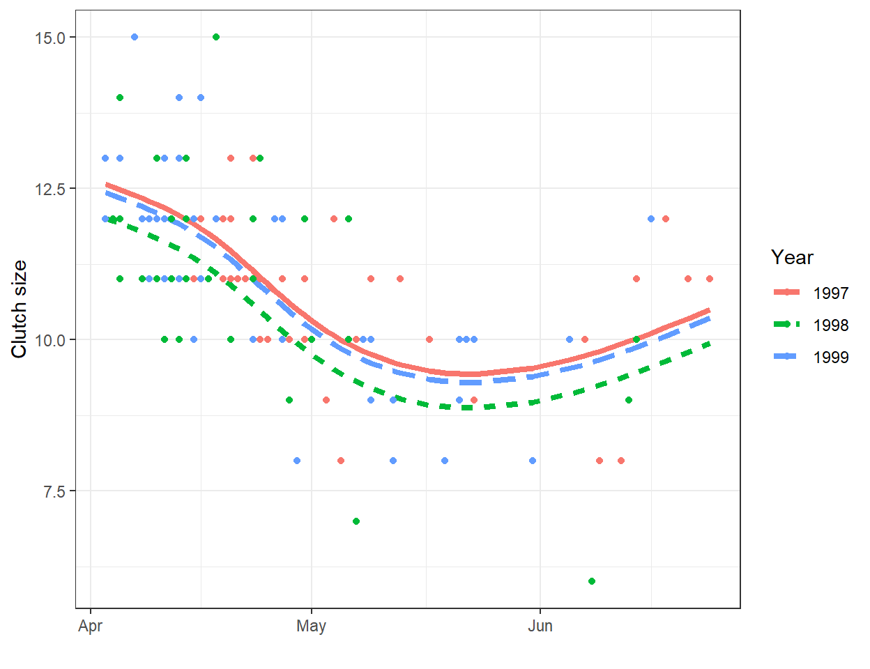
FIGURE 4.1: Clutch size of mallards nesting in nest boxes in Minnesota versus nest initiation date. Data from Zicus et al. (2003).
In the above example, the relationship between clutch size and nest initiation date was modeled using a polynomial, but other options are possible. To help understand different approaches to fitting non-linear relationships, we will begin by considering simple examples using data on plant species richness for 29 islands in the Galapagos Islands archipelago (Johnson & Raven, 1973). This section borrows heavily from Jack Weiss’s lecture notes from his Statistical Ecology course (which unfortunately are no longer accessible), but also considers additional curve fitting approaches using polynomials and regression splines.
Ecologists have long been interested in how the number of unique species (\(S\)) scales with area (\(A\)), or so called species-area curves (for an overview, see Conor & McCoy, 2013). This interest comes from both a desire to understand the underlying mechanisms that create these relationships as well as from potential applications in research design (e.g., use in developing appropriate sampling designs for describing ecological communities) and conservation and wildlife management (e.g., design of protected areas and estimation of impacts due to habitat loss). Several different statistical models have been proposed for describing species-area curves. We will consider a few of these models here, including:
- \(S_i = \beta_0 + \beta_1A_i + \epsilon_i\) (linear relationship between species and area)
- \(S_i = \beta_0 + \beta_1log(A_i) + \epsilon_i\) (linear relationship between species and log area)
- \(S_i = aA_i^b\gamma_i\), which can also be expressed on a log-log scale as \(log(S_i) = \beta_0 + \beta_1log(A_i) + \epsilon_i\)
Let’s begin by plotting the data on plant species richness relative to area in a few different ways:
p1 <- ggplot(gala, aes(x = Area, y = Species)) + geom_point(size = 3)  +
  xlab("Area") + theme_grey(base_size = 20)
p2 <- ggplot(gala, aes(x = logarea, y = Species)) + geom_point(size = 3)  +
  xlab("log(Area)") + theme_grey(base_size = 20)
p3<- ggplot(gala, aes(x = logarea, y = log(Species))) + geom_point(size = 3)  +
  xlab("log(Area)") + theme_grey(base_size = 20) + ylab("log(Species)")
gridExtra::grid.arrange(p1, p2, p3, ncol=3)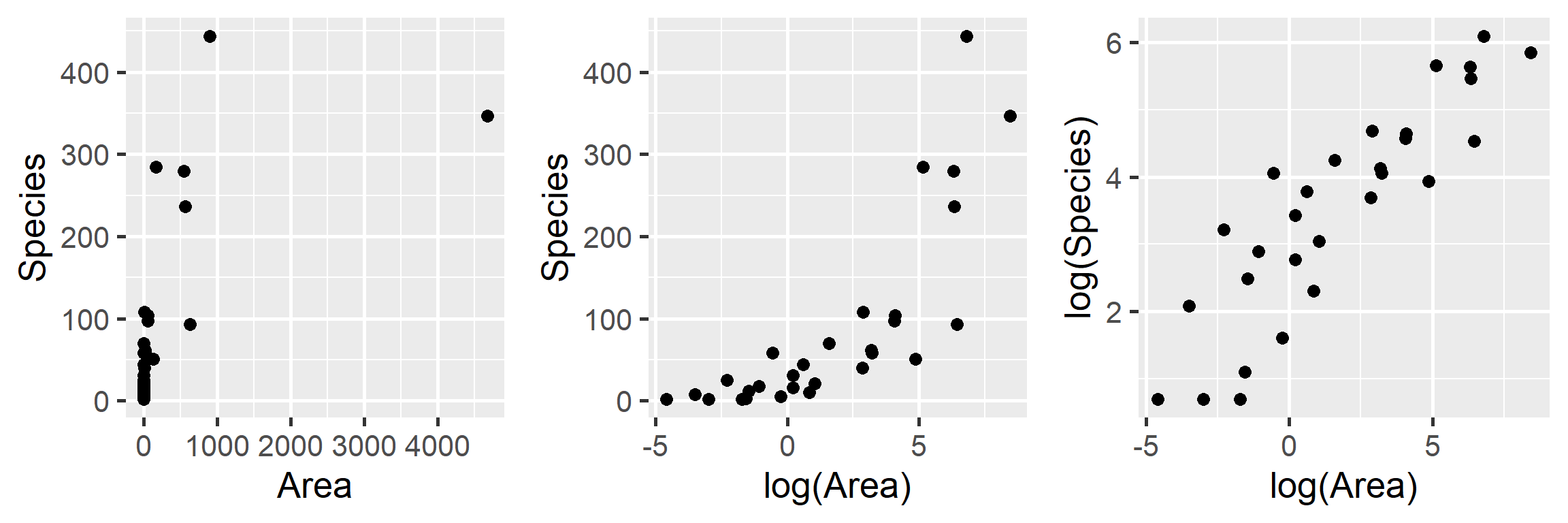
FIGURE 4.2: Plant species richness versus area for 29 islands in the Galapagos Islands archipelago. Data are from (Johnson & Raven, 1973).
We clearly see that the first two models are not appropriate as the relationship between \(S_i\) and \(A_i\) and between \(S_i\) and \(\log(A_i)\) is not linear. On the other hand, a linear model appears appropriate for describing the relationship between \(\log(S_i)\) and \(\log(A_i)\). Below, we fit this model and explore whether the assumptions of the model hold (Figure 4.3):
##
## Call:
## lm(formula = log(Species) ~ log(Area), data = gala)
##
## Residuals:
##      Min       1Q   Median       3Q      Max
## -1.44745 -0.40009  0.06723  0.51319  1.45385
##
## Coefficients:
##             Estimate Std. Error t value Pr(>|t|)
## (Intercept)  2.83384    0.15709  18.040  < 2e-16 ***
## log(Area)    0.40427    0.04121   9.811 2.13e-10 ***
## ---
## Signif. codes:  0 '***' 0.001 '**' 0.01 '*' 0.05 '.' 0.1 ' ' 1
##
## Residual standard error: 0.7578 on 27 degrees of freedom
## Multiple R-squared:  0.7809, Adjusted R-squared:  0.7728
## F-statistic: 96.25 on 1 and 27 DF,  p-value: 2.135e-10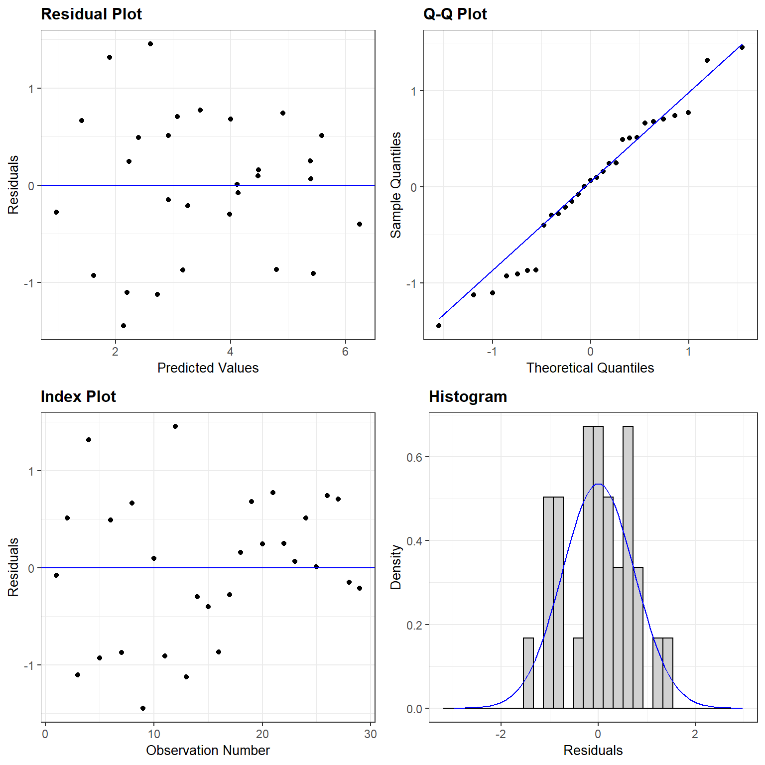
FIGURE 4.3: Residual plot for a linear model relating log plant species richness to log species area for 29 islands in the Galapagos Islands archipelago. Data are from (Johnson & Raven, 1973).
The assumptions look like they are fairly well met, suggesting that this is a reasonable model for the data-generating process.
Importantly, this model is a linear model, but for the transformed response, \(\log(S_i)\) and for the transformed predictor, \(\log(A_i)\). This brings up an important point, namely that we can use a linear modeling framework to describe non-linear relationships. By linear model framework, we mean that we have a model where the response variable can be written as a “linear combination” of parameters and predictor variables (i.e., a weighted sum of the predictor variables).
\[Y_i = \beta_0 + X_{i,1}\beta_1 + X_{i,2}\beta_2 + \ldots + \epsilon_i\]
We can accommodate non-linear relationships within a linear models framework by using:
- Transformations of \(X\) or \(Y\) or both (e.g., log(\(X\)), \(\sqrt{Y}\), \(\exp(X)\)).
- Polynomials (e.g.,\(X\) plus \(X^2\)) as predictors in our model
- Splines or piecewise polynomials that are unique to different segments of the data
I.e., the following models are still technically “linear models” and can be easily fit using lm:
\[Y_i = \beta_0 + X_i\beta_1 + X^2_i\beta_2+ \ldots + \epsilon_i\]
\[\sqrt{Y_i} = \beta_0 + log(X_i)\beta_1 + \ldots + \epsilon_i\]
Thus, these models allow us to continue to use all the same tools we have learned about (e.g., residual plots, t-tests, \(R^2\), etc). For the Galapagos data, the log transformation of \(X\) and \(Y\) results in a reasonable model for the data. The primary downside is that our model describes the relationship between the log species richness and log area. Although it is tempting to use the inverse transformation (i.e., \(\exp()\)) to allow inference back on the original scale, doing so will not preserve the mean – i.e., \(\exp(E[\log(S)]) \ne E[S]\). Furthermore, the variability about the mean will no longer be described by a normal distribution. Essentially, we have a model that assumes the errors, \(\gamma_i = \exp(\epsilon_i)\) are multiplicative and log-normally distributed (Section 9.11.2). It is also important to note that metrics used to compare models (e.g., the AIC; 8.3) are not straightforward when considering models for both the original and transformed data (i.e., \(S_i\) and \(\log(S_i)\)). We could use results from Section 9.11.2 to derive the mean back on the original scale or simulate data from our model of the data generating process to facilitate further inference. A better approach would be to use a generalized linear model appropriate for count data, which we will eventually see in Section 15. In the next sections, we will consider alternative approaches for curve fitting using polynomials and regression splines.
4.2 Polynomials
If we look at the relationship between species and log(Area) (middle panel of Figure 4.2), it appears that a quadratic function might describe the mean species-area curve well. We can explore this model using ggplot by adding geom_smooth(method="lm", formula=y~poly(x,2), se=TRUE):
ggplot(gala, aes(x=logarea, y=Species)) + geom_point(size=3)+
geom_smooth(method="lm", formula=y~poly(x,2), se=TRUE) 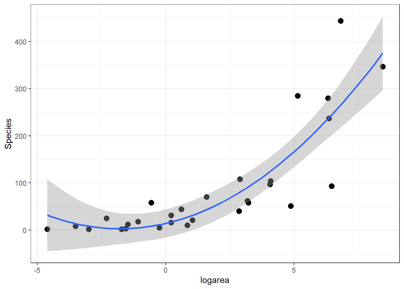
FIGURE 4.4: Quadratic polynomial fit to species-area relationship.
How can we fit this model using lm? One intuitive option would be to create a new “predictor” variable in our data set – the square of logarea and add this predictor to the linear model:
gala$logarea.squared <- gala$logarea ^ 2
lm.poly <- lm(Species ~ logarea + logarea.squared, data = gala)
summary(lm.poly)
Call:
lm(formula = Species ~ logarea + logarea.squared, data = gala)

Residuals:
     Min       1Q   Median       3Q      Max
-151.009  -27.361   -1.033   20.825  178.805

Coefficients:
                Estimate Std. Error t value Pr(>|t|)
(Intercept)      14.1530    14.5607   0.972 0.340010
logarea          12.6226     4.8614   2.596 0.015293 *
logarea.squared   3.5641     0.9445   3.773 0.000842 ***
---
Signif. codes:  0 '***' 0.001 '**' 0.01 '*' 0.05 '.' 0.1 ' ' 1

Residual standard error: 59.88 on 26 degrees of freedom
Multiple R-squared:  0.7528,    Adjusted R-squared:  0.7338
F-statistic: 39.6 on 2 and 26 DF, p-value: 1.285e-08Think-Pair-Share: Write down equations for this model using matrix notation. Include the specific elements of the design matrix for the first few observations in the data set below:
##      Island Species Endemics  Area Elevation Nearest.dist Santacruz.dist
## 1    Baltra      58       23 25.09       100          0.6            0.6
## 2 Bartolome      31       21  1.24       109          0.6           26.3
## 3  Caldwell       3        3  0.21       114          2.8           58.7
##   Adjacent.isl.area    logarea logarea.squared
## 1              1.84  3.2224694     10.38430878
## 2            572.33  0.2151114      0.04627291
## 3              0.78 -1.5606477      2.43562139
However, a second, and better, option would be to use R’s built in poly function within the call to lm.
Call:
lm(formula = Species ~ poly(logarea, 2, raw = TRUE), data = gala)

Residuals:
     Min       1Q   Median       3Q      Max
-151.009  -27.361   -1.033   20.825  178.805

Coefficients:
                              Estimate Std. Error t value Pr(>|t|)
(Intercept)                    14.1530    14.5607   0.972 0.340010
poly(logarea, 2, raw = TRUE)1  12.6226     4.8614   2.596 0.015293 *
poly(logarea, 2, raw = TRUE)2   3.5641     0.9445   3.773 0.000842 ***
---
Signif. codes:  0 '***' 0.001 '**' 0.01 '*' 0.05 '.' 0.1 ' ' 1

Residual standard error: 59.88 on 26 degrees of freedom
Multiple R-squared:  0.7528,    Adjusted R-squared:  0.7338
F-statistic:  39.6 on 2 and 26 DF,  p-value: 1.285e-08
We get the exact same fit, but as we will see later, the advantage of this approach is that various functions used to summarize the model will know that logarea and its squared term “go together.” As such, we can more easily test for the combined linear and non-linear effect of logarea (e.g., using Anova in the car package), and we can construct a meaningful component + residual plot using termplot (see e.g., Section 4.10 for more on polynomial models).
4.3 Basis functions/vectors
Lets dig deeper to see what is going on under the hood in our polynomial model:
\[Y_i = \beta_0 + \beta_2X_i + \beta_3X_i^2 + \epsilon_i\]
We see that our predicted response, \(\hat{Y}_i\) is formed by taking a weighted sum of \(X_i\) and \(X_i^2\), with the weights given by the regression coefficients for \(X_i\) and \(X_i^2\):
\[\begin{equation} \hat{Y}_i = \hat{\beta}_0 + \hat{\beta}_2X_i + \hat{\beta}_3X_i^2 \tag{4.1} \end{equation}\]
More generally, we can write any linear model as a sum of parameters \(\beta_j\) times predictors, where some of these predictors are constructed as a function of the original predictors:
\[Y_i = \sum_{j=1}^P \beta_j b_j(X_i) + \epsilon_i\]
The \(b_j(X_i)\) are called basis functions or basis vectors and are calculated using our original variable, \(X\) = logarea (Hefley et al., 2017). Our polynomial model can be written in terms of 3 basis vectors \(b_j(X_i) = 1, X_i, \mbox{ and } X_i^2\) (noting that \(1 = X^{0}\)). We plot these 3 basis vectors against logarea (our \(X\)) in Figure 4.5.
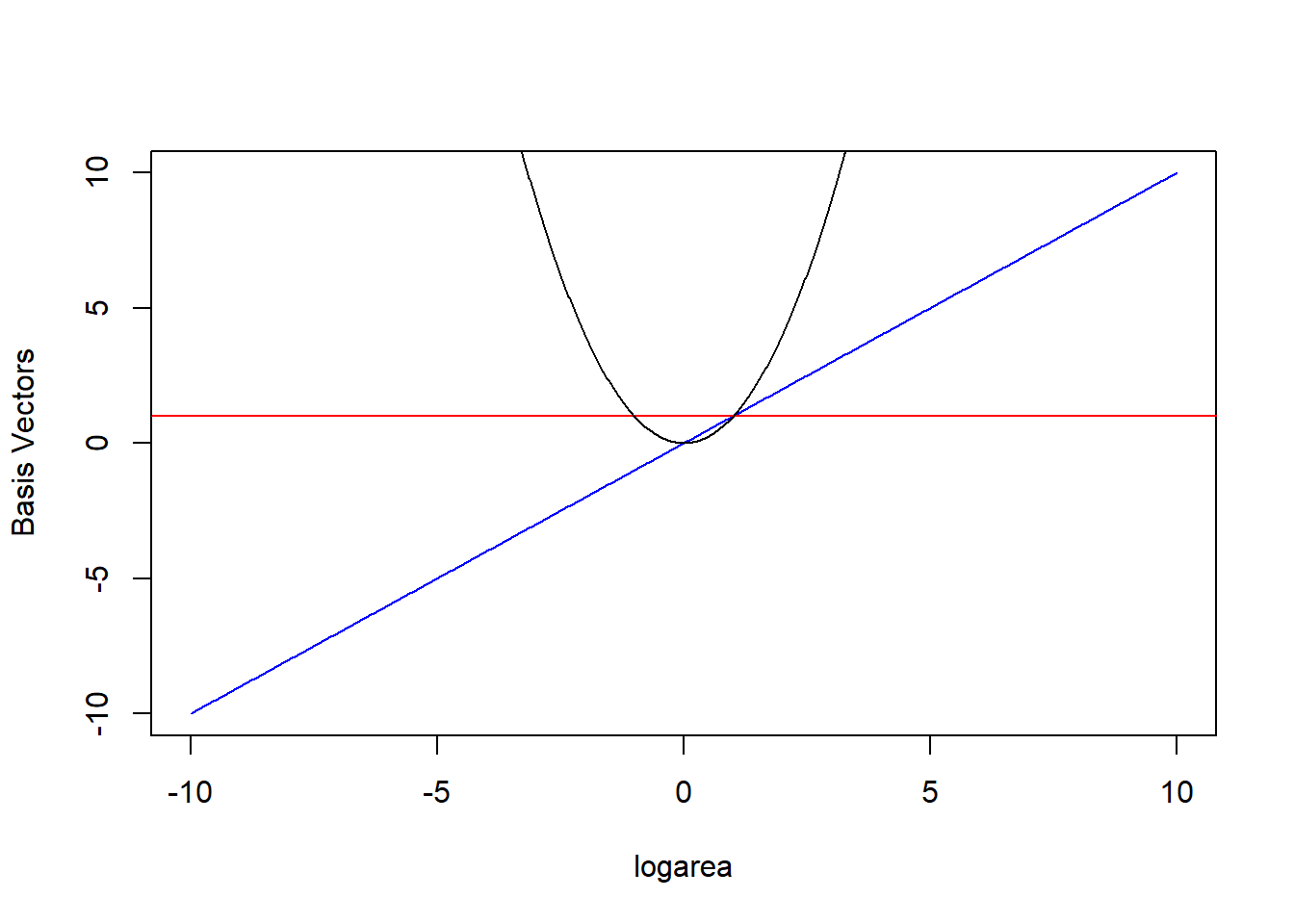
FIGURE 4.5: Set of basis vectors in the quadratic polynomial model relating plant species richness to log(Area) and log(Area)\(^2\) for 29 islands in the Galapagos Islands archipelago. Data are from (Johnson & Raven, 1973).
Lets look at our design matrix using model.matrix for the first 6 observations and also the first 6 values of logarea.
  (Intercept) poly(logarea, 2, raw = TRUE)1 poly(logarea, 2, raw = TRUE)2
1           1                     3.2224694                   10.38430878
2           1                     0.2151114                    0.04627291
3           1                    -1.5606477                    2.43562139
4           1                    -2.3025851                    5.30189811
5           1                    -2.9957323                    8.97441185
6 1 -1.0788097 1.16383029[1] 3.2224694 0.2151114 -1.5606477 -2.3025851 -2.9957323 -1.0788097We see that poly created two variables in our design matrix, \(X\) and \(X^2\) corresponding to logarea and logarea*logarea.
Our predicted species richness at any given value of logarea, \(\hat{Y}_i|X_i = E[Y_i | X_i]\) or \(\hat{Y}_i\) (as in eq. (4.1)), is formed by weighting the 3 columns of our design matrix (holding our basis vectors) by their regression coefficients:
\[E[Y_i|X_i] = \beta_01 + \beta_2X_i + \beta_3X_i^2 = 14.15 + 12.62\log(Area)_i + 3.56\log(Area)_i^2\]
In other words, \(E[Y | X]\) is given by a linear combination of the horizontal line (1, from the intercept), a line through the origin (\(X\)), and the quadratic centered on the origin (\(X^2\)) where were depicted in Figure 4.5. Also, note that a negative coefficient (i.e., weight) for \(X\) would reflect the 1-1 line about \(X = 0\) and a negative coefficient for \(X^2\) would result in a down-facing parabola. Thus, the quadratic polynomial model can fit any quadratic function, not just those that are concave up.
More generally, a polynomial of degree D is a function formed by linear combinations of the powers of its argument up to D:
\[y = \beta_0 + \beta_1x + \beta_2x^2 + \ldots + \beta_Dx^D\]
Specific polynomials:
- Linear: \(y = \beta_0 + \beta_1x\)
- Quadratic: \(y = \beta_0 + \beta_1x + \beta_2x^2\)
- Cubic: \(y = \beta_0 + \beta_1x + \beta_2x^2 + \beta_3x^3\)
- Quartic: \(y = \beta_0 + \beta_1x + \beta_2x^2 + \beta_3x^3+\beta_4x^4\)
- Quintic: \(y = \beta_0 + \beta_1x + \beta_2x^2 + \beta_3x^3+\beta_4x^4 + \beta_5x^5\)
The design matrix for a regression model with \(n\) observations and \(p\) predictors will be a matrix with \(n\) rows and \(p\) columns such that the value of the \(j^{th}\) predictor for the \(i^{th}\) observation is located in column \(j\) of row \(i\).
Design matrix for a polynomial of degree D
\[\begin{bmatrix} 1 & x_1 & x_1^2 & x_1^3 & \ldots & x_1^D \\ 1 & x_2 & x_2^2 & x_2^3 & \ldots & x_2^D \\ 1 & x_3 & x_3^2 & x_3^3 & \ldots & x_3^D \\ & & \vdots & & \\ 1 & x_n & x_n^2 & x_n^3 & \ldots & x_n^D \\ \end{bmatrix}\]
Higher order polynomials can allow for more complex patterns, but they have “global constraints” on their shape. For example, quadratic functions must eventually either increase (or decrease) as \(X\) gets both really large or small. Cubic polynomials must move in opposite directions (i.e., increase and decrease) as \(X\) gets really large versus really small and small, etc. We can gain further flexibility by combining polynomials applied separately to short segments of our data along with local constraints that ensure the different polynomials get “stitched” together in a reasonable way (i.e., by using splines).
4.4 Splines
Splines are piecewise polynomials used in curve fitting. They may seem mysterious at first, but like polynomials, they can be understood as models that weight different basis vectors constructed from predictor variables included in the model.
4.4.1 Linear splines
Linear models are often a good approximation over small ranges of \(x\). Thus, one option for modeling non-linear relationships is to “piece together” several linear models fit to short segments of the data, taking care to make sure that the “ends meet” at the boundaries of each segment.
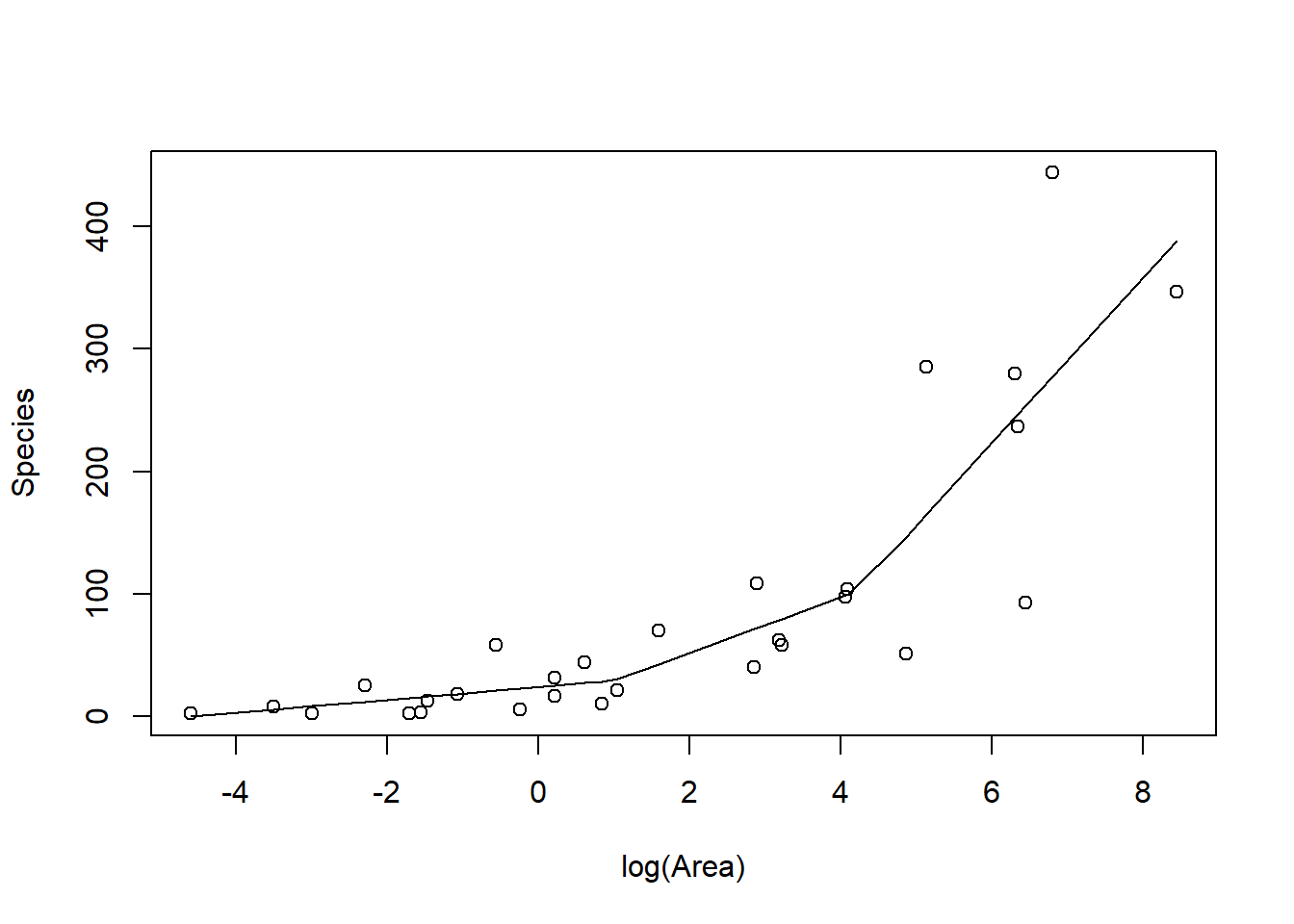
FIGURE 4.6: Piecewise linear model relating plant species richness to log(Area) for 29 islands in the Galapagos Islands archipelago. Data are from (Johnson & Raven, 1973).
The above plot was constructed by fitting a model with the effect of logarea modeled using a linear spline. A linear spline is a continuous function formed by connecting linear
segments. The points where the segments connect are called the knots of the spline.
We chose 2 knots (located at logarea = 1 and 4.2, where the relationship between Species and logarea appeared to change) and formed two basis vectors by subtracting the knot from logarea and setting the value to 0 whenever the expression was negative:
(logarea-1)\(_+\)(logarea-4.2)\(_+\)
where the \(_+\) indicates that we set the value equal to 0 when the expression was negative. Here is how we created the basis vectors in R:
gala$logarea<- log(gala$Area)
gala$logarea.1<- ifelse(gala$logarea<1, 0, gala$logarea-1)
gala$logarea.4.2<- ifelse(gala$logarea<4.2, 0, gala$logarea-4.2)
We then fit our model using lm:
##
## Call:
## lm(formula = Species ~ logarea + logarea.1 + logarea.4.2, data = gala)
##
## Residuals:
##      Min       1Q   Median       3Q      Max
## -160.691  -16.547   -4.209   13.133  166.430
##
## Coefficients:
##             Estimate Std. Error t value Pr(>|t|)
## (Intercept)   23.869     17.384   1.373   0.1819
## logarea        5.213      8.956   0.582   0.5658
## logarea.1     17.464     18.836   0.927   0.3627
## logarea.4.2   44.815     23.156   1.935   0.0643 .
## ---
## Signif. codes:  0 '***' 0.001 '**' 0.01 '*' 0.05 '.' 0.1 ' ' 1
##
## Residual standard error: 58.97 on 25 degrees of freedom
## Multiple R-squared:  0.7695, Adjusted R-squared:  0.7418
## F-statistic: 27.82 on 3 and 25 DF,  p-value: 3.934e-08
As with the polynomial model, our predicted species richness at any given value of logarea, \(\hat{Y}_i|X_i = E[Y_i | X_i]\), is formed by summing the weighted columns of our design matrix by their regression coefficients. The basis vectors, their weighted versions, and the fitted curve formed by summing the weighted basis vectors are depicted in Figure 4.7.
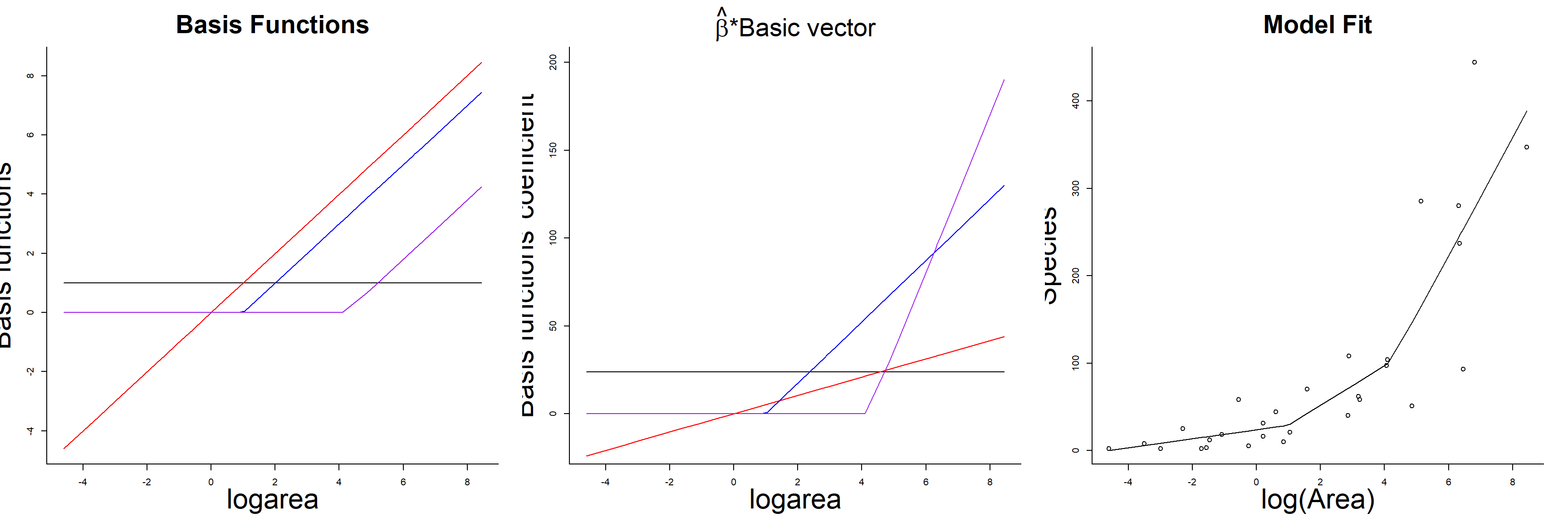
FIGURE 4.7: Basis vectors, weighted basis vectors, and predicted values formed by summing the weighted basis vectors in the linear spline model fit to species-area data.
Linear splines can sometimes be useful for modelling abrupt changes in response variables or to depict relationships where we might expect a response variable to asymptote after crossing some threshold value of the predictor variable. For example, Thompson, Johnson, Niemuth, & Ribic (2015) used linear splines with a constraint that the slope be 0 after a single knot to model the effect of disturbance from oil and gas wells on bird abundance (Figure 4.8). They compared the fits of standard linear models to the fits provided by segmented regression (Toms & Lesperance, 2003), which is essentially a spline-based model but one in which the knot location is also a free parameter to be estimated from the data. As can be seen in three of the four panels, the best-fit “lines” are a better visual fit to the data than a single straight line would be.
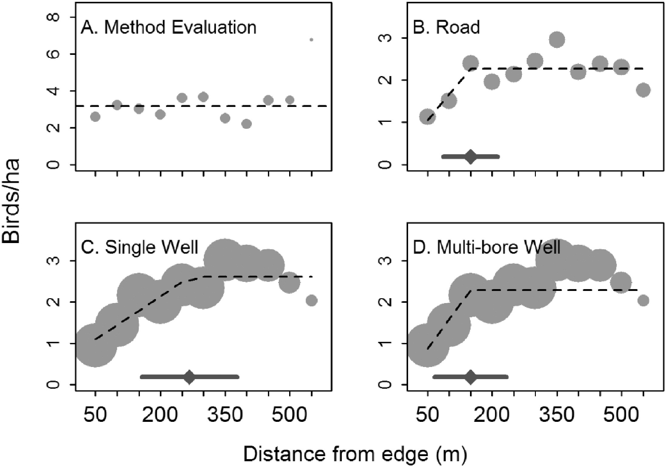
FIGURE 4.8: Figure 2 from Thompson et al. (2015) describing models used to explore the effect of oil and gas disturbance on grassland bird abundance in North Dakota.
4.4.2 Cubic regression splines
More generally, a spline of degree D is a function formed by connecting polynomial segments of degree D so that:
- the function is continuous (i.e., it is not disjointed when it hits a knot)
- the function has D-1 continuous derivatives
- the D\(^{th}\) derivative is constant between knots
Linear splines (D = 1) only ensure our function is continuous. The first derivative, which describes if the function is increasing or decreasing, is not constant. As a result, our fitted curve (Figure 4.6) looks somewhat jagged at the knot locations. In fact, the fitted model can be increasing before a knot and decreasing after it! Usually, we expect biological relationships to be smoother than this. Therefore, unless we have an expectation that \(Y\) will change drastically after crossing a threshold, we will generally benefit from approaches that result in a smoother fit to the data.
Cubic splines (D = 3) are commonly used in model fitting, and ensure that \(\hat{Y}\) and its first two derivatives are continuous everywhere (even at the knot locations). Remember, the first derivative (tells us if the function is increasing or decreasing), whereas the second derivative tells us about curvature (whether the function is concave up or down at a minimum or maximum).
There are a number of different ways of creating basis vectors that lead to piecewise cubic polynomials with continuous first and second derivatives. The simplest approach is to use truncated polynomials, which is how we created our linear spline.
The truncated polynomial of degree D associated with a knot \(\xi_k\) is the function which is equal to 0 to the left of \(\xi_k\) and equal to \((x - \xi_k)^D\) to the right of \(\xi_k\).
\[(x - \xi_k)^D_+ = \left\{ \begin{array}{ll} 0 & \mbox{if } x < \xi_k\\ (x - \xi_k)^D & \mbox{if } x \ge \xi_k \end{array} \right.\]
We can fit a model using a spline of degree D with K knots:
\[Y_i = \beta_0 +\sum_{d=1}^D \beta_DX_i^d + \sum_{k=1}^K b_k(X_i - \xi_k)^D_+ +\epsilon_i\]
The design matrix in this case is given by an \(n \times (1 + 3 + K)\) matrix with entries:
\[\begin{bmatrix} 1 & x_1 & x_1^2 & x_1^3 & (x_1 - \xi_1)^3_+ & \ldots & (x_1 - \xi_k)^3_+\\ 1 & x_2 & x_2^2 & x_2^3 & (x_2 - \xi_1)^3_+ & \ldots & (x_2 - \xi_k)^3_+\\ 1 & x_3 & x_3^2 & x_3^3 & (x_3 - \xi_1)^3_+ & \ldots & (x_3 - \xi_k)^3_+\\ & & \vdots & & \\ 1 & x_n & x_n^2 & x_n^3 & (x_n - \xi_1)^3_+ & \ldots & (x_n - \xi_k)^3_+\\ \end{bmatrix}\]
Although truncated power bases are easiest to understand, they may lead to numerical problems due to scaling issues (Perperoglou, Sauerbrei, Abrahamowicz, & Schmid, 2019). Other popular options are:
- Bsplines (
bs(x, df=)insplinespackage)
- Natural or restricted cubic splines (
ns(x, df=)insplinespackage;rcs(x,df)inrcspackage)
B-splines are numerically more stable than those based on the truncated power basis but can be poorly behaved near the edge of the data range. Natural or restricted cubic splines address this problem by assuming the model is linear before the first knot and after the last knot. A further advantage of these additional constraints is that it requires fewer basis vectors and thus, eats up fewer model degrees of freedom (\(k-1\) versus \(k-3\), where \(k\) is the number of knots). We will return to this point when we get to the section on model selection [add link].
In addition to b-splines and natural splines, cyclical splines can be used to model circular data like time of day or annual response patterns (e.g., Ditmer et al., 2015). In these cases, we would want our model to give similar predictions just before versus just after midnight or just before versus after a new year begins. Cyclical splines use basis vectors that are formed in a way that ensures these constraints are upheld. .
4.4.3 Natural cubic regression splines
To fit a model with the effect of logarea on species richness modeled using a natural cubic regression spline, we use the ns function in the spline library.
Call:
lm(formula = Species ~ ns(logarea, 3), data = gala)

Residuals:
     Min       1Q   Median       3Q      Max
-156.173  -13.819   -5.998   13.922  170.555

Coefficients:
                Estimate Std. Error t value Pr(>|t|)
(Intercept)        1.468     43.542   0.034   0.9734
ns(logarea, 3)1   47.790     45.957   1.040   0.3084
ns(logarea, 3)2  276.125    102.146   2.703   0.0122 *
ns(logarea, 3)3  381.743     45.084   8.467 8.22e-09 ***
---
Signif. codes:  0 '***' 0.001 '**' 0.01 '*' 0.05 '.' 0.1 ' ' 1

Residual standard error: 59.48 on 25 degrees of freedom
Multiple R-squared:  0.7655,    Adjusted R-squared:  0.7374
F-statistic: 27.21 on 3 and 25 DF,  p-value: 4.859e-08
We see from the output that we have estimated 4 coefficients. Lets look at the design matrix for the first few observations and a plot the different basis functions created by ns (i.e., the columns of the design matrix) versus logarea.
##    (Intercept) ns(logarea, 3)1 ns(logarea, 3)2 ns(logarea, 3)3
## 17           1      0.00000000       0.0000000       0.0000000
## 8            1     -0.07289332       0.1993098      -0.1235349
## 5            1     -0.09952908       0.2856200      -0.1770311
## 4            1     -0.12204050       0.3907838      -0.2422131
## 9            1     -0.12443447       0.4653235      -0.2884138
## 3            1     -0.12199115       0.4821792      -0.2988612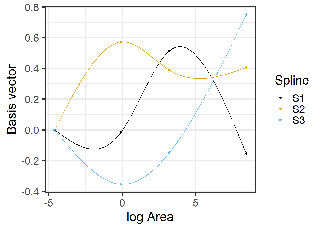
FIGURE 4.9: Basis vectors used in the fitting of the natural cubic regression spline model relating plant species richness to log(Area) for 29 islands in the Galapagos Islands archipelago. Data are from (Johnson & Raven, 1973).
The predicted species richness values are again formed by weighting the basis functions in Figure 4.9 along with the intercept. We can use ggplot to see the resulting fitted curve:
ggplot(gala, aes(x = logarea, y = Species)) + geom_point(size = 3) +
geom_smooth(method = "lm", formula = y ~ ns(x, 3), se = TRUE) 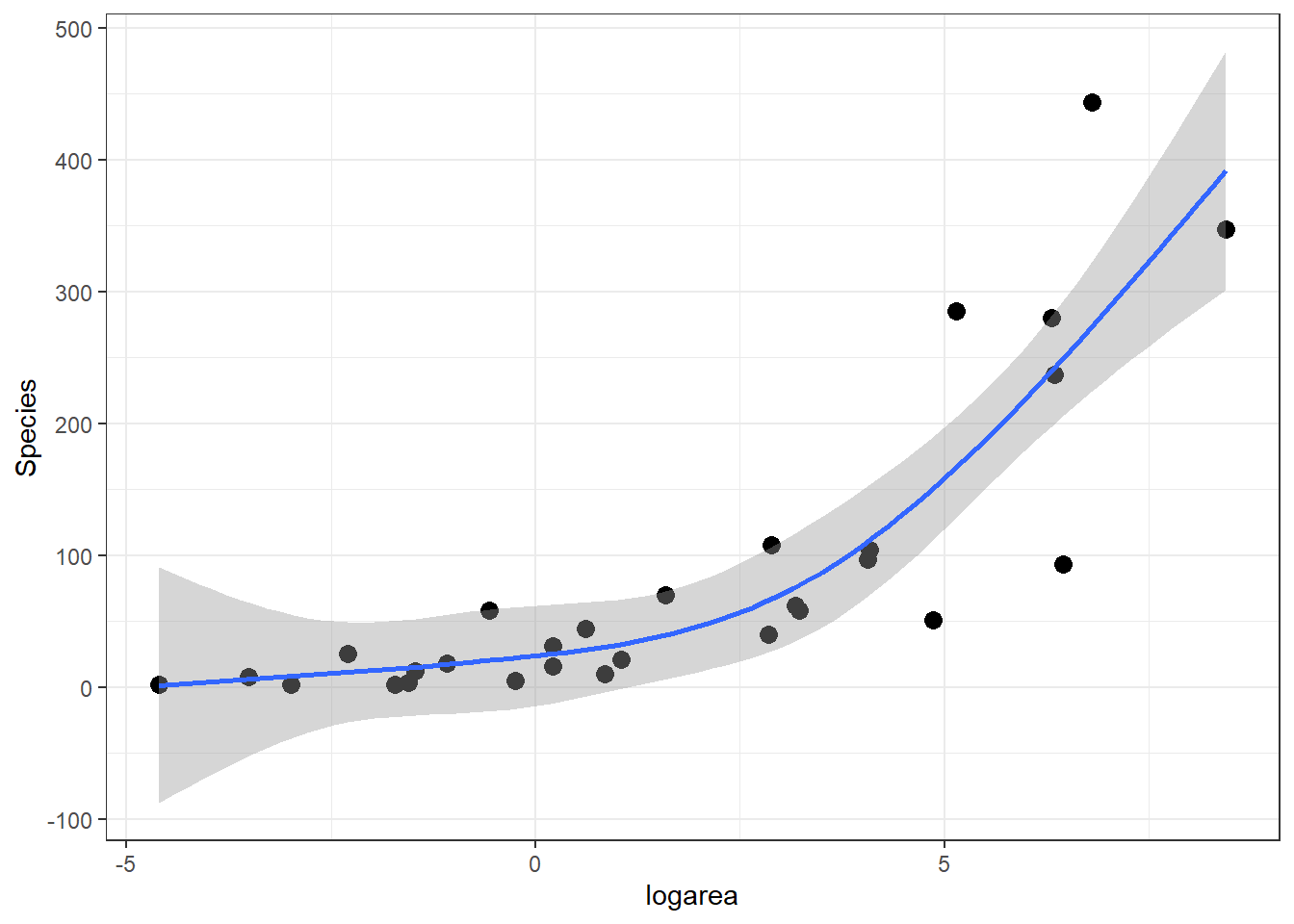
FIGURE 4.10: Predicted values from the natural cubic regression spline model relating plant species richness to log(Area) for 29 islands in the Galapagos Islands archipelago. Data are from (Johnson & Raven, 1973).
4.4.4 Number of knots and their locations
The shape of a spline can be controlled by carefully choosing the number of knots and their exact locations in order to allow greater flexibility where the trend appears to be changing quickly, while avoid overfitting in regions where the trend changes little. We could, in principle, compare models (e.g., using AIC) that have varying numbers of knots, or different knot locations. The danger here is that we would open the door to a wide range of possible models, increasing the chances we would overfit our data. Further, proper accounting of model-selection uncertainty associated with such data-driven processes can be challenging, a topic we will discuss in Section 8.
An alternative strategy is to choose a small number of knots (df), based on how much data you have and how complex you expect the relationship to be a priori (Harrell Jr, 2015). I have personally found that 2 or 3 internal knots are usually sufficient for small data sets. Also, Keele & Keele (2008), cited in Zuur et al. (2009), recommend 3 knots if \(n < 30\) and 5 knots if \(n > 100\). As for choosing the locations of the knots, we can do this using quantiles of the data (what ns does by default if you do not provide knot locations). Fortunately, models fit with cubic regression splines are usually not too sensitive to knot locations (Harrell Jr, 2015). Alternatively, you can choose to place knots in places where you expect the relationship between \(X\) and \(Y\) to be changing rapidly based on familiarity with the system.
We can see the knots chosen by ns using:
  33.33333%   66.66667%
-0.09393711 3.20877345 [1] -4.605170 8.448769The latter 2 knots are located at the outer limits of the data (remember, the model is assumed to be linear outside of this range):
## [1] -4.605170 8.4487694.5 Splines versus polynomials
We have not yet talked about how we can compare competing models, but one popular method is to use the Akaike’s Information Criterion or AIC (Akaike, 1974; Anderson & Burnham, 2004). Smaller values of AIC are generally preferable.
             df      AIC
lmfit         3 335.1547
lm.poly1.raw  4 324.4895
lm.sp         5 324.4646
lm.ns         5 324.9600
Here, we see that all of the non-linear approaches we have so far considered fit better than a linear model. Although the natural cubic regression spline and polynomial models have similar AIC values, the spline model seems to provide a better fit for especially small values of logarea (Figure 4.11). In particular, the polynomial model appears to suggest species richness will stop decreasing and actually start increasing once logarea decreases past a certain point and approaches the smallest values in our data set, which does not seem reasonable. This is an inherent limitation of quadratic polynomials, which all have to eventually point in the same direction at the extremes of the data. By contrast, splines all for more “local control” when fitting deviations from linearity.
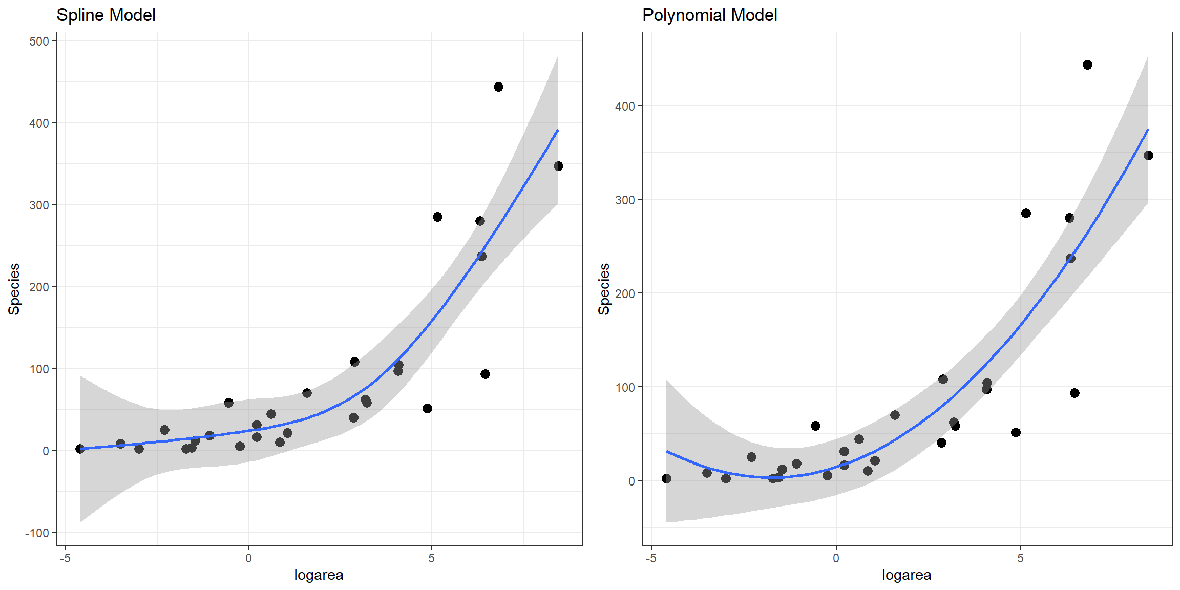
FIGURE 4.11: Comparison of predicted values from the natural cubic regression spline and polynomial models fit to plant species richness data collected from 29 islands in the Galapagos Islands archipelago. Data are from (Johnson & Raven, 1973).
4.6 Visualizing non-linear relationships
In the previous sections, we used ggplot to visualize our fitted models (e.g., Figure 4.10). This worked since our model only included a single predictor, logarea. More generally, we can use termplot to create a partial residual plot (see Section 3.13.2) depicting the effect of logarea while controlling for other predictors that may be included in the model:
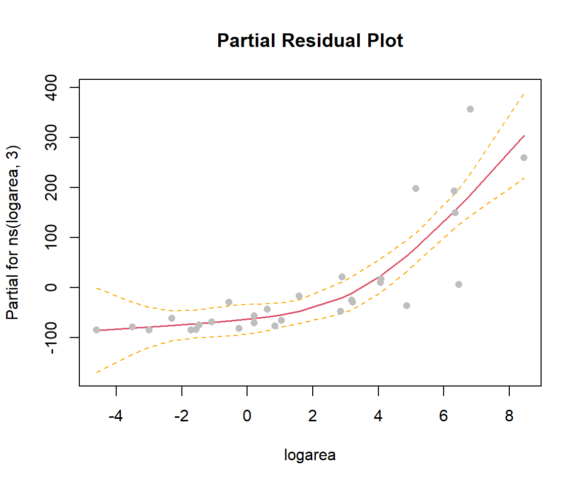
FIGURE 4.12: Partial residual plot depicting the effect of logarea on species richness in the natural cubic regression spline model fit to plant species richness data collected from 29 islands in the Galapagos Islands archipelago. Data are from (Johnson & Raven, 1973).
Another option is to use the ggeffects package (Lüdecke, 2018) to produce effect plots (see Section 3.13.3; Figure 4.13).
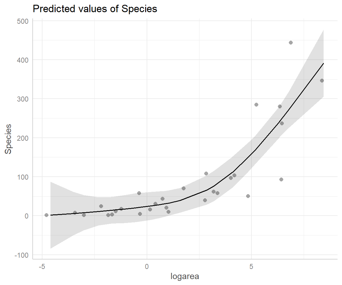
FIGURE 4.13: Partial residual plot depicting the effect of logarea on species richness in the natural cubic regression spline model fit to plant species richness data collected from 29 islands in the Galapagos Islands archipelago. Data are from (Johnson & Raven, 1973).
4.7 Generalized additive models (GAMS)
In general, non-linear models with a single predictor can be written as:
\[Y = \beta_0 + f(x_i) + \epsilon_i\]
where \(f(x_i)\) can be modeled in a variety of ways, many of which are covered in Ch. 3 of Zuur et al. (2009). Here, I briefly mention an approach based on smoothing splines, since this approach is popular among ecologists and related to the regression spline approach we covered in the last section.
Smoothing splines are constructed using lots of basis vectors (created using the same methods we saw in the last section), but the coefficients are “shrunk” towards 0 in an attempt to balance overfitting and smoothness. Although smoothing splines are perhaps easiest to understand philosophically when fitted in a Bayesian framework (they arise naturally from certain prior assumptions about the level of smoothness), they can also be implemented using penalized likelihoods, or since we have not yet covered maximum likelihood yet, penalized sums of squares:
\[PSS = \sum_{i=1}^n (y_i-\hat{y}_i)^2 + \lambda \int f^{\prime \prime}(x)dx\] or, equivalently:
\[\begin{equation} PSS = \sum_{i=1}^n (y_i-\beta_0+f(x_i))^2 + \lambda \int f^{\prime \prime}(x)dx \tag{4.2} \end{equation}\]
Here, \(f^{\prime \prime}(x)\) is the second derivative of \(f(x)\) and describes how smooth the curve is (high values are indicative of a lot of ‘wigglyness’), and \(\lambda\) is a tuning parameter that determines the penalty for `smoothness’ (larger values will result in less ‘wigglyness’, and as \(\lambda \rightarrow \infty\), \(f(x)\) will approach a straight line).
In this framework, how should we determine \(\lambda\)? Typically, this is accomplished using cross validation in which we seek to minimize the sum-of-squared prediction errors (see e.g., Section 8.7.1):
\[SSE = \frac{1}{n}\sum_{i=1}^n(Y_i - \hat{f}^{[-i]}(x_i))^2\]
where \(\hat{f}^{[-i]}(x_i)\) is the fit of the model using all observations except for observation \(i\). In practice, there are mathematical expressions/approximations that allow us to choose \(\lambda\) without fitting the model \(n\) times.
We can fit a GAM model, allowing for a non-linear relationship between species richness and log(Area) using the gam function in mgcv package (Wood, 2004; S. N Wood, 2017):
Family: gaussian
Link function: identity

Formula:
Species ~ s(logarea)

Parametric coefficients:
            Estimate Std. Error t value Pr(>|t|)
(Intercept)    87.34      11.11   7.864 2.76e-08 ***
---
Signif. codes:  0 '***' 0.001 '**' 0.01 '*' 0.05 '.' 0.1 ' ' 1

Approximate significance of smooth terms:
             edf Ref.df     F p-value
s(logarea) 2.465  3.107 24.86  <2e-16 ***
---
Signif. codes:  0 '***' 0.001 '**' 0.01 '*' 0.05 '.' 0.1 ' ' 1

R-sq.(adj) =  0.734   Deviance explained = 75.8%
GCV = 4062.7  Scale est. = 3577.3    n = 29
The small p-value for s(logarea) tells us that the relationship between logarea and Species is statistically significant and used approximately 2.5 effective model degrees of freedom (edf). Note, however, because GAMs use the data to choose \(\lambda\) (and effective model degrees of freedom), the p-values can be misleading; Simon N Wood (2017) suggests p-values are often too small and should be multiplied by a factor of 2 (see also discussion in Ch 3.6 of Zuur et al., 2009).
To understand the model, it is best to explore the fit of the model using the associated plot function.
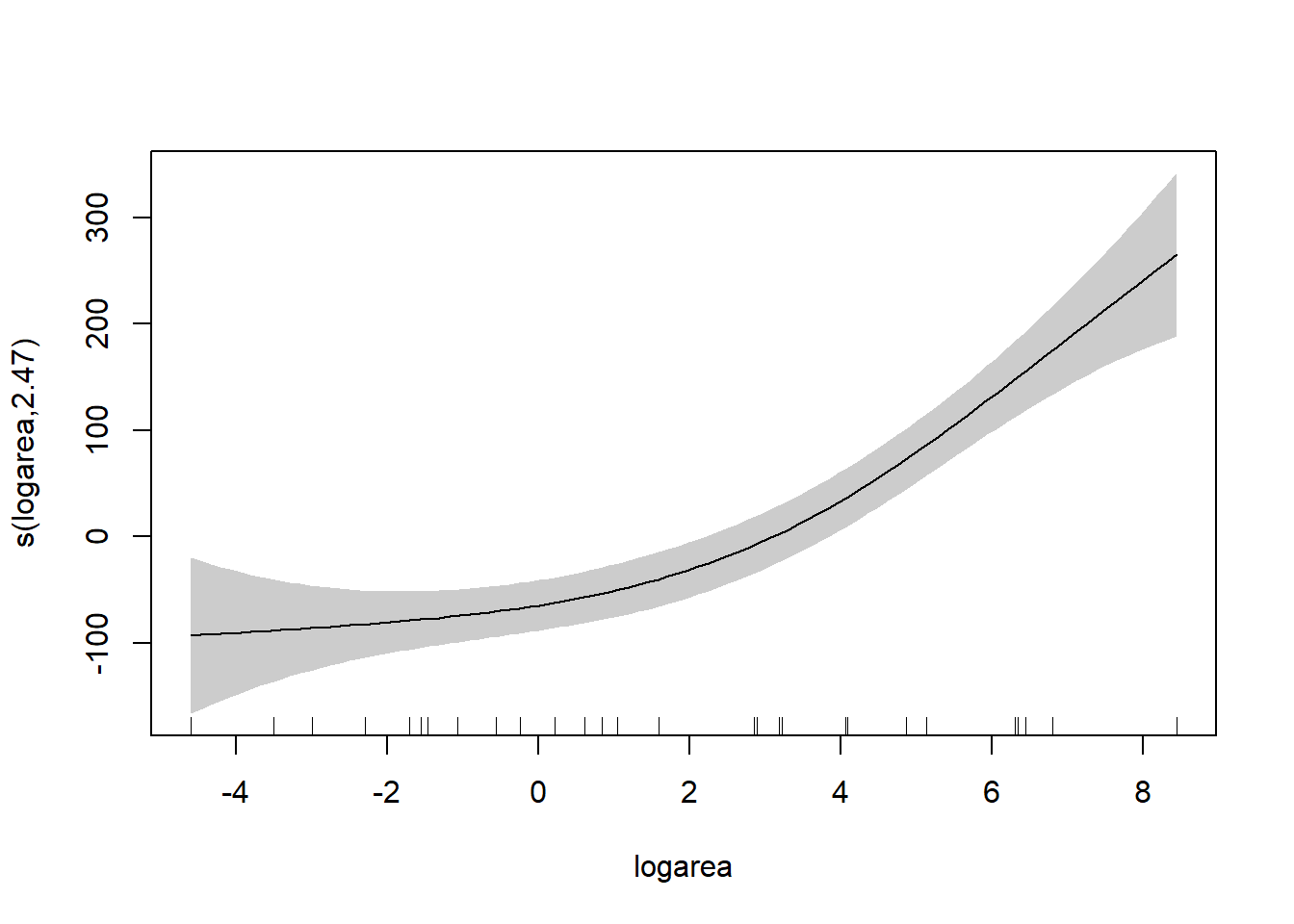
Besides the assumption of linearity, which we have relaxed, we otherwise have the same distributional assumptions as in any linear regression model, namely, that residuals are normally distributed with constant variance. We can use the gam.check function to explore whether these assumptions are met.
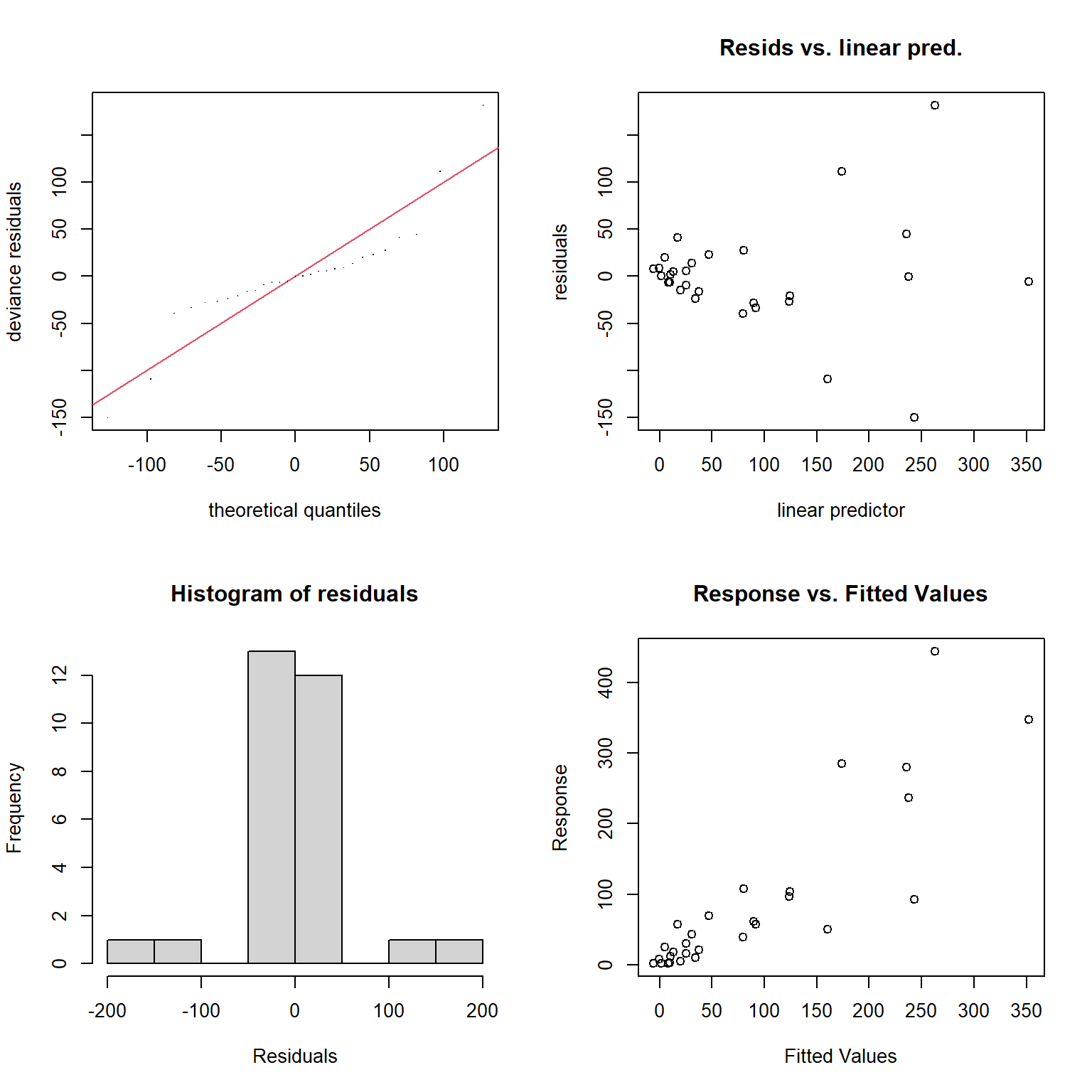
FIGURE 4.14: Model diagnostics for the fitted GAM model produced using the gam.check function.
Method: GCV   Optimizer: magic
Smoothing parameter selection converged after 6 iterations.
The RMS GCV score gradient at convergence was 0.0002855077 .
The Hessian was positive definite.
Model rank =  10 / 10

Basis dimension (k) checking results. Low p-value (k-index<1) may
indicate that k is too low, especially if edf is close to k'.

             k'  edf k-index p-value
s(logarea) 9.00 2.47    1.43    0.98
The plots produced by the gam.check function (Figure 4.14) suggest the variance of the residuals seems to increase with \(\hat{Y}\) (top right panel), and they also do not appear to be Normally distributed (left panels). As with the RIKZ data, we are modeling a species count and would likely be better off using a distribution other than the Normal distribution (as we will see when we get to generalized linear models in Section 14).
As mentioned previously, the model is fit by creating a large number of basis vectors and then estimating the coefficients for those basis vectors using the penalized sum of squares in equation (4.2). The large p-value associated with the “Basis dimension check” suggests that the default choice for number of basis vectors (9 here) was sufficient for modeling the relationship between logarea and Species. To demystify GAMS, we highly recommend Noam Ross’s online and free GAM class.
4.8 Generalizations to multiple non-linear relationships
What if you want to allow for multiple non-linear relationships? We can add multiple ns terms to our model or use multiple smoothing splines (see Zuur et al., 2009 Chapter 3; Simon N Wood, 2017). We could also consider other basis functions to fit `smooth surfaces’ (allowing for interactions between variables), including tensor splines, thin plate splines, etc… (see Simon N Wood, 2017). It is also possible to include interactions with regression splines or fit separate smooth for each value of a categorical variable (see Zuur et al., 2009 Chapter 3).
4.9 Non-Linear models with a mechanistic basis
Sometimes we may have a theoretical model linking \(X\) and \(Y\). For example, we may want to assume \(Y \sim f(x,\beta)\), where \(f(x,\beta)\) is given by, for example:
- The Ricker model for stock-recruitment: \(S_{t+1} = S_te^{r(1-\beta S_t)}\)
- A typical predator-prey relationship: \(f(N) = \frac{aN}{1+ahN}\)
Some of these models can be fit using non-linear least squares in R (e.g., using the nls function in base R). Alternatively, we will eventually learn how to fit custom models using Maximum likelihood and Bayesian methods (see Section 10.6).
4.10 Aside: Orthogonal polynomials
Standard polynomial-basis vectors can cause numerical issues when fitting linear models due to differences in scale. For example, if \(X = 100\), then \(X^3 = 1,000,000\). As a result, the coefficients weighting the X and X3 terms to be on very different scales, which can make them hard to estimate accurately. In such cases, centering and scaling \(X\) prior to deriving polynomial terms (i.e., creating a new variable for use in the model by subtracting the mean of \(X\) and diving through by the standard deviation of \(X\)) can help.
Alternatively, we can use orthogonal polynomials created usingpoly(raw=FALSE) (the default). This will create a different set of basis functions for fitting a quadratic polynomial, but one that leads to an identical fit as the raw polynomial model. We can verify this by comparing predicted values and statistical tests for the effect of logarea modeled with both raw and orthogonal polynomials.
lm.poly.raw<-lm(Species~poly(logarea,2, raw=TRUE), data=gala)
lm.poly.orth<-lm(Species~poly(logarea,2), data=gala)
plot(fitted(lm.poly.raw), fitted(lm.poly.orth), xlab="Normal Polynomials",
     ylab="orthogonal Polynomials")
abline(0,1)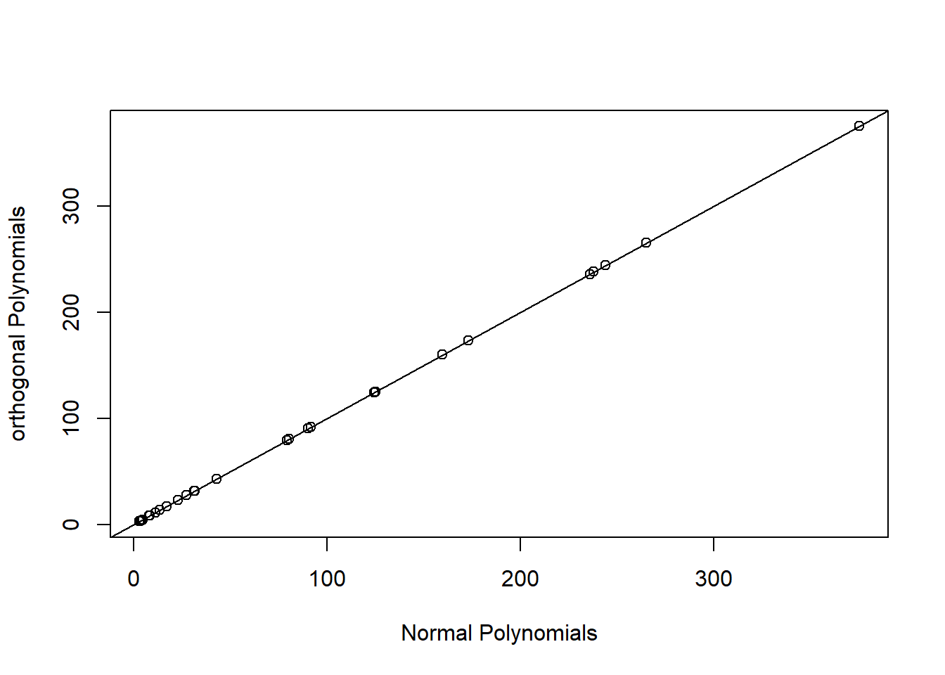
FIGURE 4.15: Predicted values for models using raw and orthogonal polynomials, demonstrating their equivalence.
.
Anova Table (Type II tests)

Response: Species
                             Sum Sq Df F value    Pr(>F)
poly(logarea, 2, raw = TRUE) 283970  2  39.596 1.285e-08 ***
Residuals                     93232 26
---
Signif. codes:  0 '***' 0.001 '**' 0.01 '*' 0.05 '.' 0.1 ' ' 1
Anova Table (Type II tests)
Response: Species
Sum Sq Df F value Pr(>F)
poly(logarea, 2) 283970 2 39.596 1.285e-08 ***
Residuals 93232 26
---
Signif. codes: 0 '***' 0.001 '**' 0.01 '*' 0.05 '.' 0.1 ' ' 1Lets look at the basis vectors used to model the effect of logarea in the two models (Figure 4.16):
##               1         2
## [1,] -0.3425801 0.4850314
## [2,] -0.2828395 0.2782420
## [3,] -0.2550617 0.1950582## [,1] [,2]
## [1,] -4.605170 21.207592
## [2,] -3.506558 12.295948
## [3,] -2.995732 8.974412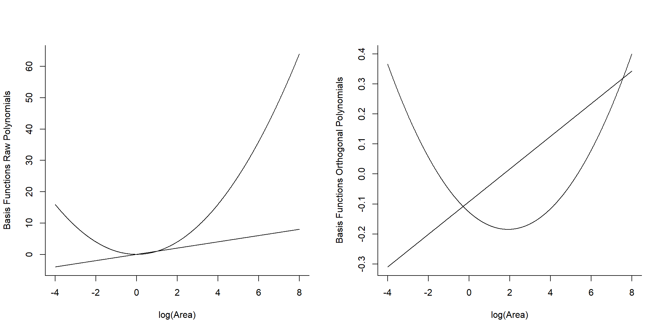
FIGURE 4.16: Basic vectors used to fit raw and orthogonal polynomial models.
We see that raw and orthogonal polynomials use different basis vectors. Both sets of vectors span the set of all quadratic polynomial functions, meaning that we can form any quadratic polynomial using a weighted sum of either set of basis vectors (for more, see Hefley et al., 2017). So, while they result in different parameter estimates, the models and fitted values are identical!