Chapter 5 Generalized least squares (GLS)
Learning Objectives
- Learn how to use generalized least squares (GLS) to model data where \(Y_i | X_i\) is normally distributed, but the variance of the residuals is not constant and may depend on one or more predictor variables.
There are a few reasons why I like to cover this class of model:
There are many data sets where a linear model would be appropriate except for the assumption that the variance of the residuals is constant. Thus, I have found GLS models to be a very useful tool to have in one’s toolbox.
The GLS framework can be used to model data where the residuals are not independent due to having multiple measurements on the same sample unit (see Section 18). In addition, it can be used to model data that are temporally or spatially correlated (though we will not cover those methods in this book).
Lastly, GLS models will give us additional practice with describing models using a set equations. Linear models allow us to write the mean of the Normal distribution as a function of one or more predictor variables. GLS models require that we also consider that the variance of the Normal distribution may depend on one or more predictor variables.
5.1 Generalized least squares (GLS): non-constant variance
In Chapter 1, we considered models of the following form:
\[Y_i = \beta_0 + X_{1i}\beta_1 + X_{2i}\beta_2 + \ldots X_{pi}\beta_p+\epsilon_i\]
where the \(\epsilon_i\) were assumed to be independent, normally distributed, and have constant variance. This allowed us to describe our model for the data using:
\[\begin{gather} Y_i \sim N(\mu_i, \sigma^2) \nonumber \\ \mu_i = \beta_0 + X_{1i}\beta_1 + X_{2i}\beta_2 + \ldots X_{pi}\beta_p \nonumber \end{gather}\]
In this chapter, we will consider models where the variance also depends on covariates, leading to the following model specification below:
\[\begin{gather} Y_i \sim N(\mu_i, \sigma_i^2) \nonumber \\ \mu_i = \beta_0 + X_{1i}\beta_1 + X_{2i}\beta_2 + \ldots X_{pi}\beta_p \nonumber \\ \sigma^2_i = f(Z_i; \delta) \nonumber \end{gather}\],
where \(\sigma_i\) is written as a function, \(f(Z_i; \tau)\), of predictor variables, \(Z\), and additional variance parameters, \(\delta\); \(Z\) may overlap with or be distinct from the predictors used to model the mean (i.e., \(X\)).
The nlme package in R (Pinheiro, Bates, DebRoy, Sarkar, & R Core Team, 2021) has several built in functions for modeling the variance, some of which are highlighted below:
varIdent: \(\sigma^2_i = \sigma^2_g\) (allowing for different variances for each level of a categorical variable, \(g\))
varFixed,varPower,varExp, andvarConstPower: \(\sigma^2_i = \sigma^2X_i\), \(\sigma^2 |X_i|^{2\delta}\), \(\sigma^2e^{2\delta X_i}\), and \(\sigma^2 (\delta_1 + |X_i|^{\delta})^2\) (models where the variance scales with a continuous covariate, \(X\))
- \(\sigma^2_i= \sigma^2E[Y_i|X_i]^{2\theta} = \sigma^2(\beta_0 + X_{1i}\beta_1 + X_{2i}\beta_2 + \ldots X_{pi}\beta_p)^{2\theta}\) (models where the variance depends on the mean)
We will explore these three different options in the next few sections. For a thorough description of available choices in nlme, see Pinheiro & Bates (2006) and Zuur et al. (2009).
5.2 Variance heterogeneity among groups: T-test with unequal variances
Let’s begin by considering a really simple example, namely extending the linear model used to test for differences in the mean jaw lengths of male and female jackals from Section 3.5.1 to allow for unequal variances. Specifically, we will consider the following model:
\[\begin{gather} Y_i \sim N(\mu_{sex_i}, \sigma^2_{sex_i}) \tag{5.1} \end{gather}\]
We can fit this model using the gls function in the nlme package (Pinheiro et al., 2021). To do so, we specify the variance model using the weights argument:
The argument’s name, weights, reflects the fact that the variance function is used to weight each observation when fitting the model. Specifically, estimates of regression parameters are obtained by minimizing:
\[\begin{gather} \sum_{i = 1}^n \frac{(Y - \mu_i)^2}{2\sigma^2_i} \nonumber \end{gather}\]
In other words, instead of minimizing the sum-of-squared errors, we minimize a weighted version where each observation is weighted by the inverse of its variance.
There are a number of different variance models that we can fit, each with its own variance function. In this case, we have used the varIdent variance function, which allows the variance to depend on a categorical variable, in this case, sex. The model is parameterized using multiplicative factors, \(\delta_g\), for each group \(g\) (i.e., each unique level of the categorical variable), with \(\delta_g\) set equal to 1 for a reference group:
\[\begin{gather} \sigma^2_i = \sigma^2\delta^2_{sex_i} \tag{5.2} \end{gather}\]
Let’s use the summary function to inspect the output of our GLS model so that we can match our parameter estimates to the parameters in our model (eq. (5.1)):
## Generalized least squares fit by REML
##   Model: jaws ~ sex
##   Data: jawdat
##        AIC      BIC    logLik
##   102.0841 105.6456 -47.04206
##
## Variance function:
##  Structure: Different standard deviations per stratum
##  Formula: ~1 | sex
##  Parameter estimates:
##         M         F
## 1.0000000 0.6107279
##
## Coefficients:
##             Value Std.Error   t-value p-value
## (Intercept) 108.6 0.7180211 151.24903  0.0000
## sexM          4.8 1.3775993   3.48432  0.0026
##
##  Correlation:
##      (Intr)
## sexM -0.521
##
## Standardized residuals:
##         Min          Q1         Med          Q3         Max
## -1.72143457 -0.70466510  0.02689742  0.76657633  1.77522940
##
## Residual standard error: 3.717829
## Degrees of freedom: 20 total; 18 residualThink-pair-share: Use the output above to estimate the mean jaw length for males and females. Based on the output, do you think the jaw lengths are more variable for males or females?
Like the lm function, gls will, by default, use effects coding to model differences between males and females in their mean jaw length:
\[\mu_i = \beta_0 + \beta_1 \text{I(sex=male)}_i\]
If you have forgotten how to estimate the mean for males and females from the output of the model, I suggest reviewing Section 3.5.1.
To get estimates of the variances for males and females, note that the residual standard error will be used to estimate \(\sigma\) in equation (5.2), i.e., \(\hat{\sigma} =\) 3.72. Also, note that the estimates of the \(\delta\)’s are given near the top of the summary output. We see that whereas female serves as our reference group when estimating coefficients associated with the mean part of the model, male serves as our reference group in the variance model and is thus assigned a \(\delta_{m} = 1\). For females, we have \(\delta_{f} = 0.61\). Putting the pieces together and using equation (5.2), we have:
- for males: \(\hat{\sigma}_i^2 = \hat{\sigma}^2\delta_m^2 = \hat{\sigma}^21 =\) 13.82.
- for females: \(\hat{\sigma}_i^2 = \hat{\sigma}^2\delta_{f}^2 = \hat{\sigma}^20.61=\) 5.16.
We can verify that these estimates are reasonable by calculating the variance of the observations for each group:
## # A tibble: 2 x 2
##   sex   `var(jaws)`
##   <chr>       <dbl>
## 1 F            5.16
## 2 M           13.8
5.2.1 Comparing the GLS model to a linear model
Is the GLS model an improvement over a linear model? Good question. It may depend on the purpose of your model. It does allow us to relax the assumption of constant variance. And, it allows us to assign higher weights to observations that are associated with parts of the predictor space that are less variable. This may lead to precision gains when estimating regression coefficients if our variance model is a good one. Lastly, it may provide a better model of the data generating process, which can be particularly important when trying to generate accurate prediction intervals (see Section 5.4).
At this point, you may be wondering about whether or not we can formally compare the two models. The answer is that we can, but with some caveats that will be discussed in Section 18.11. One option is to use AIC, which will give a conservative test, meaning that it will tend to “prefer” simpler models. We won’t formally define AIC until after we have learned about maximum likelihood. Yet, AIC is commonly used to compare models and can, for now, be viewed as a measure of model fit that penalizes for model complexity. In order to make this comparison, we will need to first fit the linear model using the gls function. By default, gls uses restricted maximum likelihood to estimate model parameters rather than maximum likelihood (these differences will be discussed when we get to Section 18.11). In this case, AIC is nearly identical for the two models.
##           df      AIC
## lm_ttest   3 102.1891
## gls_ttest  4 102.0841
We will further discuss model selection strategies in the context of GLS models in Section 5.5 and more generally in Section 8.
5.2.2 Aside: Parameterization of the model
When fitting the model, the gls function actually parameterizes the variance model on the log scale, which is equivalent in this case to:
\[\begin{gather} log(\sigma_i) = log(\sigma) + log(\delta)\text{I(sex = female)}_i \tag{5.3} \end{gather}\]
We can see this be extracting the parameters that are actually estimated:
##  varStruct     lSigma
## -0.4931037  1.3131400
If we exponentiate the second parameter, we get \(\hat{\sigma}\):
##   lSigma
## 3.717829
If we exponentiate the first parameter, we get the multiplier of \(\sigma\) for females, \(\delta_f\):
## varStruct
## 0.6107279
And, we get the standard deviation for females by exponentiating the sum of the two parameters:
## varStruct
## 2.270582## varStruct
## 5.155543Why is this important? When fitting custom models, it often helps to have parameters that are not constrained - i.e., they can take on any value between \(-\infty\) and \(\infty\). Whereas \(\sigma\) must be \(>0\), \(\log(\sigma)\) can take on any value. We will return to this point when we see how to use built in optimizers in R to fit custom models using maximum likelihood (Section 10.4.4).
5.3 Variance increasing with \(X_i\) or \(\mu_i\)
In many cases, you may encounter data for which the variance increases as a function of one of the predictor variables or as a function of the predicted mean. We will next consider one such data set, which comes from a project I worked on when I was a Biometrician at the Northwest Indian Fisheries Commission.
Aside: Many of the tribes in the Pacific Northwest and throughout North America signed treaties with the US government that resulted in the cessation of tribal lands but with language that acknowledged their right to hunt and fish in their usual and accustomed areas. Many tribal salmon fisheries were historically located near the mouth of rivers or further up stream, whereas commercial and recreational fisheries often target fish at sea. Salmon spend most of their adult life in the ocean only coming back to rivers to spawn, and then, for most salmon species, to die. As commercial fisheries became more prevalent and adopted technologies that increased harvest efficiencies, and habitat became more fragmented and degraded, many salmon stocks became threatened and endangered in the mid 1900’s. With fewer fish coming back to spawn, the State of Washington passed laws aimed at curtailing tribal harvests. The tribes fought for their treaty rights in court, winning a series of cases. The most well known court case, the Boldt Decision in 1974, reaffirmed that the treaty tribes, as sovereign nations, had the right to harvest fish in their usual and accustomed areas. Furthermore, it established that the tribes would be allowed 50% of the harvestable catch. The Northwest Indian Fisheries Commission was created to provide scientific and policy support to treaty tribes in Washington, and to help with co-management of natural resources within ceded territories.
In this section, we will consider data used to manage sockeye salmon (Oncorhynchus nerka) that spawn in the Fraser River system of Canada; the fishery is also important to the tribes in Washington State and US commercial fisherman. A variety of data are collected and used to assess the strength of salmon stocks, including “test fisheries” in the ocean that measure catch per unit effort, in-river counts of fish, and counts of egg masses (“reds”) from fish that spawn. We will consider data collected in-river from a hydroacoustic counting station operated by the Pacific Salmon Commission near the town of Mission (Figure 5.1) as well as estimates of the number of fish harvested up-stream or that eventually spawn (referred to as the spawning escapement). Systematic differences between estimates of fish passing by Mission (\(X\)) and estimates of future harvest plus spawning escapement (\(Y\)) are attributed to in-river mortalities, which may correlate with environmental conditions (e.g., stream temperature and flow). Fishery managers rely on models that forecast future harvest and spawning escapement from in-river measurements of temperature/discharge and estimates of fish passing the hydroacoustic station at Mission (Cummings, Hague, Patterson, & Peterman, 2011). If in-river mortalities are projected to be substantial, managers may reduce the allowable catch to increase the chances of meeting spawning escapement goals.

FIGURE 5.1: Map of Canada with an inset of the Fraser River Watershed of British Columbia from (Cooke et al., 2009)(https://onlinelibrary.wiley.com/doi/10.1111/j.1752-4571.2009.00076.x), published under a CC By 4.0 license. The number of salmon passing Mission is estimated using hydroacoustic counts.
Salmon in the Fraser river system spawn in several different streams and are typically managed based on stock aggregates formed by grouping stocks that travel through the river at similar “run” times. Typically, models would be constructed separately for each stock aggregate. For illustrative purposes, however, we will consider models fit to data from all stocks simultaneously.
# Load here package so can use a relative path to read data
library(here)
# Read in escapement data
sdata<-read.csv(here("data", "Sockeyedata.csv"), header=T)

# re-order rows to make it easier to plot results
xo<-order(sdata$MisEsc)
sdata<-sdata[xo,]
We will begin by considering a model without any in-river predictors and just focus on the relationship between the estimated number of salmon passing Mission (MisEsc) and the estimated number of fish spawning at the upper reaches of the river + in-river catch above Mission (SpnEsc). Let’s begin by graphing the data:
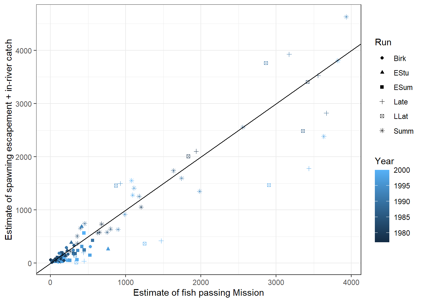
FIGURE 5.2: Summed catch and spawning escapement of Fraser Rivers sockeye salmon plotted against an estimate of the number of fish passing Mission. The black line is a 1-1 line which might be expected if there were no in-river mortalities above Mission.
From Figure 5.2 we see that: a) the two counts are highly correlated, b) there appear to be more observations below the 1-1 line than above it, as we might expect if there was significant in-river mortality, and c) the variability about the 1-1 line increases with the size of the counts. If we fit a least-squares regression line to the data and plot the residuals, we will see a “fan shape” indicating that the variance increases with the number of fish passing Mission (Figure 5.3). The Q-Q plot and histogram of residuals also suggests that there are several large residuals, more than you would expect if the residuals came from a Normal distribution with constant variance.
lmsockeye <- lm(SpnEsc ~ MisEsc, data = sdata)
ggResidpanel::resid_panel(lmsockeye, plots = c("resid", "qq", "hist"), nrow = 1)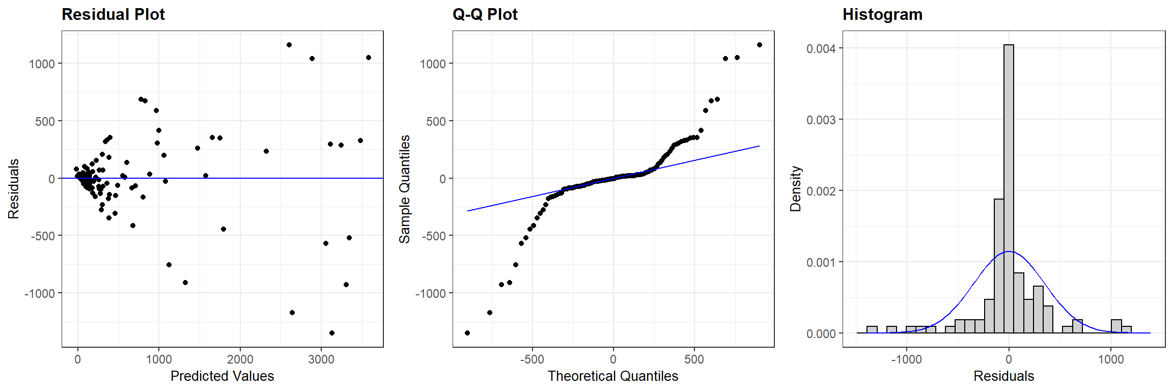
FIGURE 5.3: Residual plots for a linear model relating the estimated number of sockeye salmon passing Mission (MisEsc) to the estimated number of fish spawning at the upper reaches of the river + in-river catch above Mission (SpnEsc).
5.3.1 Variance increasing with \(X_i\)
One option for modeling data like these where the variance increases with the mean is to log both the response and predictor variable. Alternatively, we could attempt to model the variance as a function of the count at Mission. Some options include:
- Fixed variance model: \(\sigma^2_i = \sigma^2\text{MisEsc}_i\)
- Power variance model: \(\sigma^2_i = \sigma^2|\text{MisEsc}_i|^{2\delta}\)
- Exponential variance model: \(\sigma^2_i = \sigma^2e^{2\delta MisEsc_i}\)
- Constant + power variance model: \(\sigma^2_i = \sigma^2(\delta_1 + |\text{MisEsc}_i|^{\delta_2})^2\)
Before exploring these different options, it is important to note a few of their characteristics. The fixed variance model does not require any additional parameters but will only work if the covariate takes on only positive values since the \(\sigma^2_i\) must be positive. The other options do not have this limitation, but note that the power variance model can only be used if the predictor does not take on the value of 0. Pinheiro & Bates (2006) also suggest that the constant + power model tends to do better than the power model when the variance covariate takes on values close to 0. Lastly, note that several of the variance models are “nested”. Setting \(\delta = 0\) in the power variance model or the exponential variance model gets us back to the standard linear regression setting; setting \(\delta = 0.5\) in the power variance model gets us back to the fixed variance model; setting \(\delta_1 = 1\) and \(\delta_2 = 0\) in the constant + variance model gets us back to a linear regression model.
Below, we demonstrate how to fit each of these models to the salmon data:
fixedvar <- gls(SpnEsc ~ MisEsc, weights = varFixed(~ MisEsc), data = sdata)
varpow <- gls(SpnEsc ~ MisEsc, weights = varPower(form = ~ MisEsc), data = sdata)
varexp <- gls(SpnEsc ~ MisEsc, weights = varExp(form = ~ MisEsc), data = sdata)
varconstp <- gls(SpnEsc ~ MisEsc, weights = varConstPower(form = ~ MisEsc), data = sdata)
We also refit the linear model using the gls function. We then compare the models using AIC:
##           df      AIC
## lmsockeye  3 1614.925
## fixedvar   3 1459.525
## varpow     4 1446.861
## varexp     4 1482.668
## varconstp  5 1421.523
We find the constant + power variance function has the lowest AIC. Let’s look at the summary of this model:
## Generalized least squares fit by REML
##   Model: SpnEsc ~ MisEsc
##   Data: sdata
##        AIC     BIC    logLik
##   1421.523 1434.98 -705.7614
##
## Variance function:
##  Structure: Constant plus power of variance covariate
##  Formula: ~MisEsc
##  Parameter estimates:
##     const     power
## 119.49037   1.10369
##
## Coefficients:
##                 Value Std.Error   t-value p-value
## (Intercept) -6.122849  8.644421 -0.708301  0.4803
## MisEsc       0.828173  0.052627 15.736618  0.0000
##
##  Correlation:
##        (Intr)
## MisEsc -0.666
##
## Standardized residuals:
##         Min          Q1         Med          Q3         Max
## -2.03554341 -0.68214833 -0.03890184  0.61977181  2.85039770
##
## Residual standard error: 0.172081
## Degrees of freedom: 111 total; 109 residual
We see that \(\hat{\sigma} = 0.17\), \(\hat{\delta}_1 = 119.49\) and \(\hat{\delta}_2 = 1.10\). Thus, our model for the variance is given by:
\[\begin{gather} \hat{\sigma}^2_i = 0.17^2(119.49 + |\text{MisEsc}_i|^{1.10})^2 \nonumber \end{gather}\]
So, AIC suggests this is our best model, but how do we know that it is a reasonable model and not just the best of a crappy set of models? One thing we can do is plot standardized residuals versus fitted values. Specifically, if we divide each residual by \(\hat{\sigma}_i\), giving \((Y_i - \hat{Y}_i)/\hat{\sigma}_i\), we should end up with standardized residuals that have approximately constant variance:
sig2i <- 0.172081*(119.49037 + abs(sdata$MisEsc)^1.10369)
sdata <- sdata %>%
  mutate(fitted = predict(varconstp),
         stdresids  = (SpnEsc - predict(varconstp))/sig2i)
We can then plot standardized residuals versus fitted values to determine if we have a reasonable model for the variance.
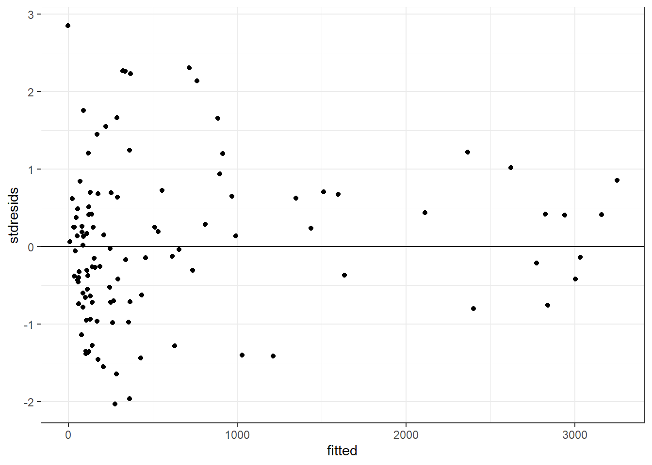
FIGURE 5.4: (ref:plotgls1)
Although there appears to be more scatter in the left size of the plot, there are also more observations in this region. We could also look at a Q-Q plot of the standardized residuals:
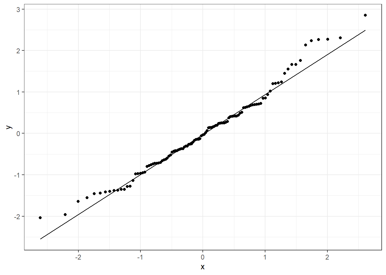
FIGURE 5.5: Q-Q plot of standardized residuals for the constant + power variance model relating the estimated number of sockeye salmon passing Mission (MisEsc) to the estimated number of fish spawning at the upper reaches of the river + in-river catch above Mission (SpnEsc).
Although it is instructive to calculate the standardized residuals “by hand”, they can also be accessed via resid(varconstp, type = "normlized"), and a plot of standardized residuals versus fitted values can be created using plot(modelobject) as demonstrated below:
##          [,1]       [,2]
## 80 2.85039770 2.85039838
## 86 0.06174022 0.06174023
## 28 0.61705145 0.61705141
5.3.2 Extension to multiple groups
The variance functions from the last section can also be extended to allow for separate variance parameters associated with each level of a categorical predictor. For example, we could specify a power variance model that is unique to each aggregated spawning run (Run) using varPower(form = ~ MiscEsc | Run):
varconstp2 <- gls(SpnEsc ~ MisEsc, weights = varConstPower(form = ~ MisEsc | Run),
                  data = sdata)
summary(varconstp2)
## Generalized least squares fit by REML
## Model: SpnEsc ~ MisEsc
## Data: sdata
## AIC BIC logLik
## 1422.534 1462.904 -696.267
##
## Variance function:
## Structure: Constant plus power of variance covariate, different strata
## Formula: ~MisEsc | Run
## Parameter estimates:
## Birk ESum EStu LLat Late Summ
## const 145.5274085 0.000023687 5.870824e-07 0.01278235 831.506521 552.0347558
## power 0.9884561 1.090556985 1.121713e+00 1.11926759 1.031333 0.9761924
##
## Coefficients:
## Value Std.Error t-value p-value
## (Intercept) -5.338079 6.264157 -0.852162 0.396
## MisEsc 0.846292 0.044241 19.128985 0.000
##
## Correlation:
## (Intr)
## MisEsc -0.646
##
## Standardized residuals:
## Min Q1 Med Q3 Max
## -1.8507998 -0.7866583 -0.1026722 0.6805132 2.0956061
##
## Residual standard error: 0.2111618
## Degrees of freedom: 111 total; 109 residualIn this case, we see that we get separate variance parameters for each aggregated stock, and the parameters appear to differ quite a bit depending on the aggregation. Yet, AIC appears to slightly favor the simpler model:
##            df      AIC
## varconstp   5 1421.523
## varconstp2 15 1422.534
5.3.3 Variance depending on \(\mu_i\)
With more complicated models that include multiple predictors that influence the mean, it is sometimes useful to model the variance not as a function of one or more predictor variables, but rather as a function of the mean itself (Pinheiro & Bates, 2006; Mech, Fieberg, & Barber-Meyer, 2018). Specifically:
\[\begin{gather} Y_i \sim N(\mu_i, \sigma_i^2) \nonumber \\ \mu_i = \beta_0 + \beta_1X_i \nonumber \\ \sigma^2_i = \mu_i^{2\delta} \nonumber \end{gather}\]
This model can be fit using varPower(form = ~ fitted(.)). I was unable to get this model to converge when using the full data set, but demonstrate its use for modeling just the early summer aggregation:
varmean <- gls(SpnEsc ~ MisEsc, weights = varPower(form = ~ fitted(.)),
                  data = subset(sdata, Run=="ESum"))
summary(varmean)
## Generalized least squares fit by REML
## Model: SpnEsc ~ MisEsc
## Data: subset(sdata, Run == "ESum")
## AIC BIC logLik
## 260.2083 264.5725 -126.1042
##
## Variance function:
## Structure: Power of variance covariate
## Formula: ~fitted(.)
## Parameter estimates:
## power
## 1.540548
##
## Coefficients:
## Value Std.Error t-value p-value
## (Intercept) 21.632043 8.875419 2.437298 0.0233
## MisEsc 0.591687 0.100345 5.896532 0.0000
##
## Correlation:
## (Intr)
## MisEsc -0.823
##
## Standardized residuals:
## Min Q1 Med Q3 Max
## -1.5456716 -0.6159292 -0.1371156 0.3850583 2.1805075
##
## Residual standard error: 0.02768571
## Degrees of freedom: 24 total; 22 residual5.4 Approximate confidence and prediction intervals
The generic predict function works with models fit using gls, but it will not return standard errors as it does for models fit using lm with the additional arguement, se.fit = TRUE. In addition, for many applications, we may be interested in obtaining prediction intervals. This section will illustrate how we can use matrix multiplication to calculate confidence and prediction intervals for our chosen Sockeye salmon model.
Think-pair-share: Consider the role these models might play in management. Do you think managers of the sockeye salmon fishery will be more interested in confidence intervals or prediction intervals?
Recall the difference between confidence intervals and prediction intervals from Chapter 1.8. Confidence intervals capture uncertainty surrounding the average value of \(Y\) at any given set of predictors, whereas a prediction interval captures uncertainty regarding a particular value of \(Y\) at a given value of \(X\). In the Sockeye Salmon example, above, managers are most likely interested in forming a prediction interval that is likely to capture the size of the salmon run in a particular year. Thus, we need to be able to calculate a prediction interval for \(Y|X\). Managers may also be interested in describing average trends across years using confidence intervals for the mean.
For a confidence interval, we need to estimate:
\[var(\hat{E}[Y|X]) = var(\hat{\beta}_0 + \hat{\beta}_1X)\]
i.e., we need to quantify our uncertainty regarding the regression line.
For a prediction interval, we need to estimate:
\[var(\hat{Y}_i|X_i) = var(\hat{\beta}_0 + \hat{\beta}_1X_i+ \epsilon_i)\]
i.e., we need to quantify both the uncertainty associated with the regression line and variability about the line.
Aside: to derive appropriate confidence and prediction intervals, we will need to leverage a bit of statistical theory, some of which was covered in Section 3.11. In particular, it helps to know that statistics such as means, sums, regression coefficients will be normally distributed if our sample size, \(n\), is “large” (thanks to the Central Limit Theorem!) Further, if the vector \((X, Y) \sim N(\mu, \Sigma)\), then for constants \(a\) and \(b\), \(aX+bY\) will be \(N(\widetilde\mu, \widetilde\Sigma)\) with:
- \(\widetilde\mu = E(aX + bY) = aE(X)+bE(Y)\)
- \(\widetilde\Sigma = var(aX + bY) = a^2var(X)+b^2var(Y)+2abcov(X,Y)\), where \(cov(X,Y)\) describes how \(X\) and \(Y\) covary. If \(cov(X,Y)\) is positive, then we expect high values of \(X\) to be associated with high values of \(Y\).
As we saw in Section 3.11, and we will further demonstrate below, matrix multiplication offers a convenient way to calculate means and variances of linear combinations of random variables (e.g., \(aX + bY\)).
We can begin by calculating predicted values for each observation in our data set by multiplying our design matrix by the estimated regression coefficients:
\[\hat{E}[Y|X]= \begin{bmatrix} 1 & \text{MscEsc}_1\\ 1 & \text{MscEsc}_2\\ \vdots & \vdots\\ 1 & \text{MscEsc}_n\\ \end{bmatrix}\begin{bmatrix} \hat{\beta}_0\\ \hat{\beta}_1\\ \end{bmatrix}=\begin{bmatrix} \hat{\beta}_0 + \text{MscEsc}_1\hat{\beta}_1\\ \hat{\beta}_0 + \text{MscEsc}_2\hat{\beta}_1\\ \vdots \\ \hat{\beta}_0 + \text{MscEsc}_n\hat{\beta}_1\\ \end{bmatrix},\]
# Design matrix for our observations
xmat <- model.matrix(~ MisEsc, data=sdata)

# Regression coefficients
betahat<-coef(varconstp)

# Predictions
sdata$SpnEsc.hat <- predict(varconstp)
cbind(head(xmat%*%betahat), head(sdata$SpnEsc.hat))
## [,1] [,2]
## 80 -1.153813 -1.153813
## 86 10.440605 10.440605
## 28 23.691368 23.691368
## 85 31.973095 31.973095
## 4 36.942131 36.942131
## 20 36.942131 36.942131The variance for the \(i^{th}\) prediction is given by:
\[var(\hat{E}[Y|\text{MscEsc}_1]) = var(\hat{\beta}_0 + \hat{\beta}_1 \text{MscEsc}_1) = var(\hat{\beta}_0) + \text{MscEsc}_1^2var(\hat{\beta}_1) + 2\text{MscEsc}_1cov(\hat{\beta}_0,\hat{\beta}_0)\]
We can calculate this variance using matrix multiplication. Let:
\[\hat{\Sigma} =\begin{bmatrix} var(\hat{\beta}_0) & cov(\hat{\beta}_0,\hat{\beta}_1)\\ cov(\hat{\beta}_0,\hat{\beta}_1) & var(\hat{\beta}_1) \\ \end{bmatrix}\]
Then, we have:
\[\begin{bmatrix} 1 & \text{MscEsc}_1\\ \end{bmatrix} \hat{\Sigma}\begin{bmatrix} 1 \\ \text{MscEsc}_1\\ \end{bmatrix}=var(\hat{\beta}_0) + \text{MscEsc}_1^2var(\hat{\beta}_1) + 2\text{MscEsc}_1cov(\hat{\beta}_0,\hat{\beta}_0)\]
Furthermore, if we calculate \(X \hat{\Sigma}X'\), where \(X\) is our design matrix, we will end up with a matrix that contains all of the variances along the diagonal and covariances between the predicted values on the off-diagonal. We can then pull off the diagonal elements (the variances), take their square root to get standard errors, and then take \(\pm 1.645SE\) to form point-wise 90% confidence intervals for the line at each value of \(X\).
We can access \(\hat{\Sigma}\) using the vcov function. Also, note that we can transpose a matrix in R using t(matrix):
# Sigma^
Sigmahat <- vcov(varconstp)

# var/cov(beta0 + beta1*X)
varcovEYhat<-xmat%*%Sigmahat%*%t(xmat)

# Pull off the diagonal elements and take their sqrt to
# get SEs that quantify uncertainty associated with the line
SEline <- sqrt(diag(varcovEYhat))
We then plot the points, fitted line, and a confidence interval for the line:
# Confidence interval for the mean
sdata$upconf <- sdata$SpnEsc.hat + 1.645 * SEline
sdata$lowconf <- sdata$SpnEsc.hat - 1.645 * SEline
p1 <- ggplot(sdata, aes(MisEsc, SpnEsc)) + geom_point() +
  geom_line(aes(MisEsc, SpnEsc.hat)) +
  geom_line(aes(MisEsc, lowconf), col = "red", lty = 2) +
  geom_line(aes(MisEsc, upconf), col = "red", lty = 2) +
  xlab("Estimate at Mission") + ylab("Estimate of C+Spawners")
p1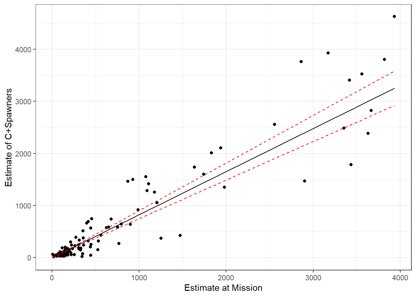
FIGURE 5.6: Predictions for the catch and spawning escapement based no the count of sockeye salmon at Mission. A 95% confidence interval for the mean is given by the red dotted lines.
For prediction intervals, we need to calculate:
\[var(\hat{Y}_i|X_i) = var(\hat{\beta}_0 + \hat{\beta}_1\text{MisEsc}_i+ \epsilon_i)\]
We will approximate this expression with:
\[var(\hat{Y}_i|X_i) \approx \widehat{var}(\hat{\beta}_0 + \hat{\beta}_1\text{MisEsc}_i) + \hat{\sigma}^2_i = X\hat{\Sigma}X^{\prime} + \hat{\sigma}^2_i,\]
where \(\hat{\sigma}_i\) is determined by our variance function and is equal to \(\hat{\sigma}^2_i = 0.17^2(119.49 + |\text{MisEsc}_i|^{1.10})^2\) for the constant + power variance model. We have already calculated \(\hat{\sigma}_i\) for all of the observations in our data set and stored it the variable sig2i. We put the different pieces together an plot the prediction intervals below:
# Approx. prediction interval, ignoring the uncertainty in theta
varpredict <- SEline ^ 2 + sig2i ^ 2
sdata$pupconf <- sdata$SpnEsc.hat + 1.645 * sqrt(varpredict)
sdata$plowconf <- sdata$SpnEsc.hat - 1.645 * sqrt(varpredict)
ggplot(sdata, aes(MisEsc, SpnEsc)) + geom_point() +
  geom_line(aes(MisEsc, SpnEsc.hat)) +
  geom_line(aes(MisEsc, lowconf), col = "red", lty = 2) +
  geom_line(aes(MisEsc, upconf), col = "red", lty = 2) +
  geom_line(aes(MisEsc, plowconf), col = "blue", lty = 2) +
  geom_line(aes(MisEsc, pupconf), col = "blue", lty = 2) +
  xlab("Estimate at Mission") + ylab("Estimate of C+Spawners")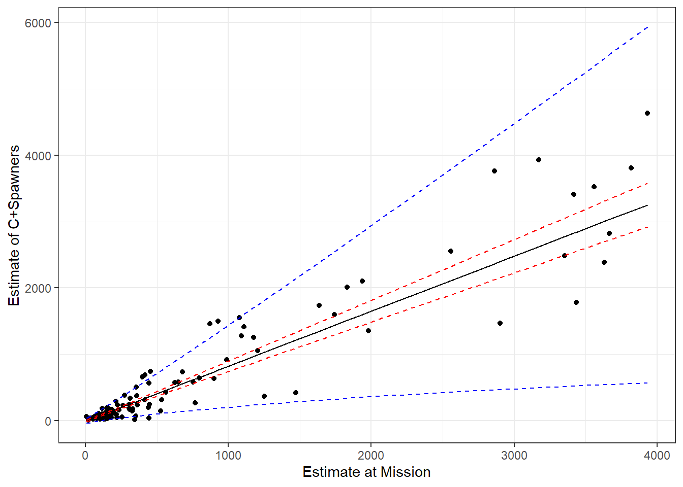
FIGURE 5.7: Predictions for the catch and spawning escapement based no the count of sockeye salmon at Mission. Blue and red lines depict 95% prediction and confidence intervals, respectively.
Before concluding, we note that these confidence and prediction intervals are approximate in that they rely on asymptotic Normality (due to the Central Limit Theorem), and they ignore uncertainty in the variance parameters.
5.5 Modeling strategy
By consider models for both the mean and variance, we have just increased the flexibility (and potential complexity) of our modeling approach. Our simple examples involved very few predictors, but what if we are faced with a more difficult challenge of choosing among many potential predictors for the mean and also multiple potential models for the variance? It is easy to fall into a trap of more and more complicated data-driven model selection, the consequences of which we will discuss in Chapter 8. My general recommendation would be to include any predictor variables in the model for the mean that you feel are important for addressing your research objectives (see Sections 6, 7, and 8 for important considerations). You might start by fitting a linear model and inspect the residuals to see if the assumptions of linear regression hold. Importantly, you could do this without even looking at the estimated coefficients and their statistical significance. Plotting the residuals versus fitted values and versus different predictors may lead you to consider a different variance function. You might then fit one or more variance models and inspect plots of standardized residuals versus fitted values to see if model assumptions are better met. You might also consider comparing models using AIC. Again, this could all be done without looking at whether the regression coefficients are statistically significant to avoid biasing your conclusions in favor of finding signifant results.